This vignette demonstrates the basics of running a dyngen simulation. If you haven’t done so already, first check out the installation instructions in the README.
Step 1: Define backbone and other parameters
A dyngen simulation can be started by providing a backbone to the
initialise_model() function. The backbone of a
dyngen model is what determines the overall dynamic process
that a cell will undergo during a simulation. It consists of a set of
gene modules, which regulate eachother in such a way that expression of
certain genes change over time in a specific manner.
library(tidyverse)
library(dyngen)

set.seed(1)

backbone <- backbone_bifurcating()
config <-
  initialise_model(
    backbone = backbone,
    num_tfs = nrow(backbone$module_info),
    num_targets = 500,
    num_hks = 500,
    verbose = FALSE
  )
# the simulation is being sped up because rendering all vignettes with one core
# for pkgdown can otherwise take a very long time
set.seed(1)

config <-
  initialise_model(
    backbone = backbone,
    num_cells = 1000,
    num_tfs = nrow(backbone$module_info),
    num_targets = 50,
    num_hks = 50,
    verbose = FALSE,
    download_cache_dir = tools::R_user_dir("dyngen", "data"),
    simulation_params = simulation_default(
      total_time = 1000,
      census_interval = 2,
      ssa_algorithm = ssa_etl(tau = 300 / 3600),
      experiment_params = simulation_type_wild_type(num_simulations = 10)
    )
  )
plot_backbone_statenet(config)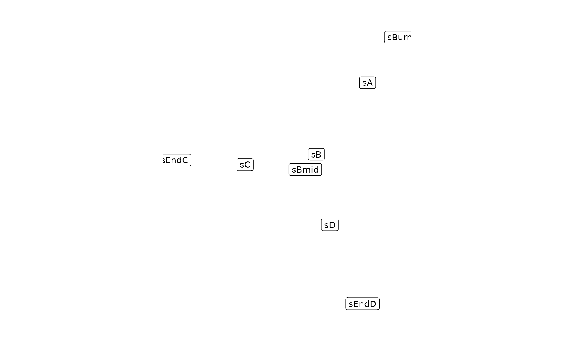
plot_backbone_modulenet(config)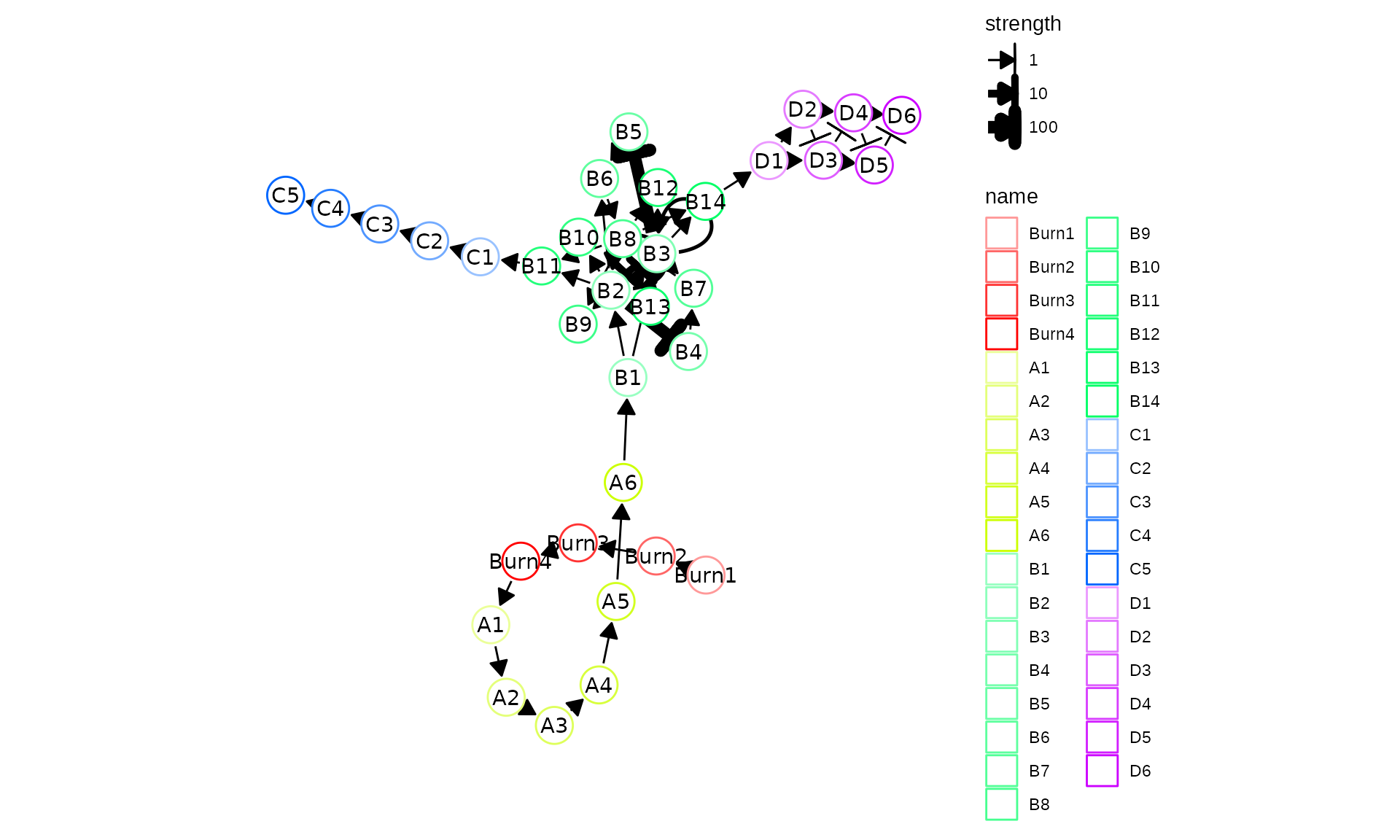
For backbones with all different sorts of topologies, check
list_backbones():
##  [1] "bifurcating"             "bifurcating_converging"
##  [3] "bifurcating_cycle"       "bifurcating_loop"
##  [5] "binary_tree"             "branching"
##  [7] "consecutive_bifurcating" "converging"
##  [9] "cycle"                   "cycle_simple"
## [11] "disconnected"            "linear"
## [13] "linear_simple"           "trifurcating"
Step 2: Generate transcription factors (TFs)
Each gene module consists of a set of transcription factors. These can be generated and visualised as follows.
model <- generate_tf_network(config)
plot_feature_network(model, show_targets = FALSE)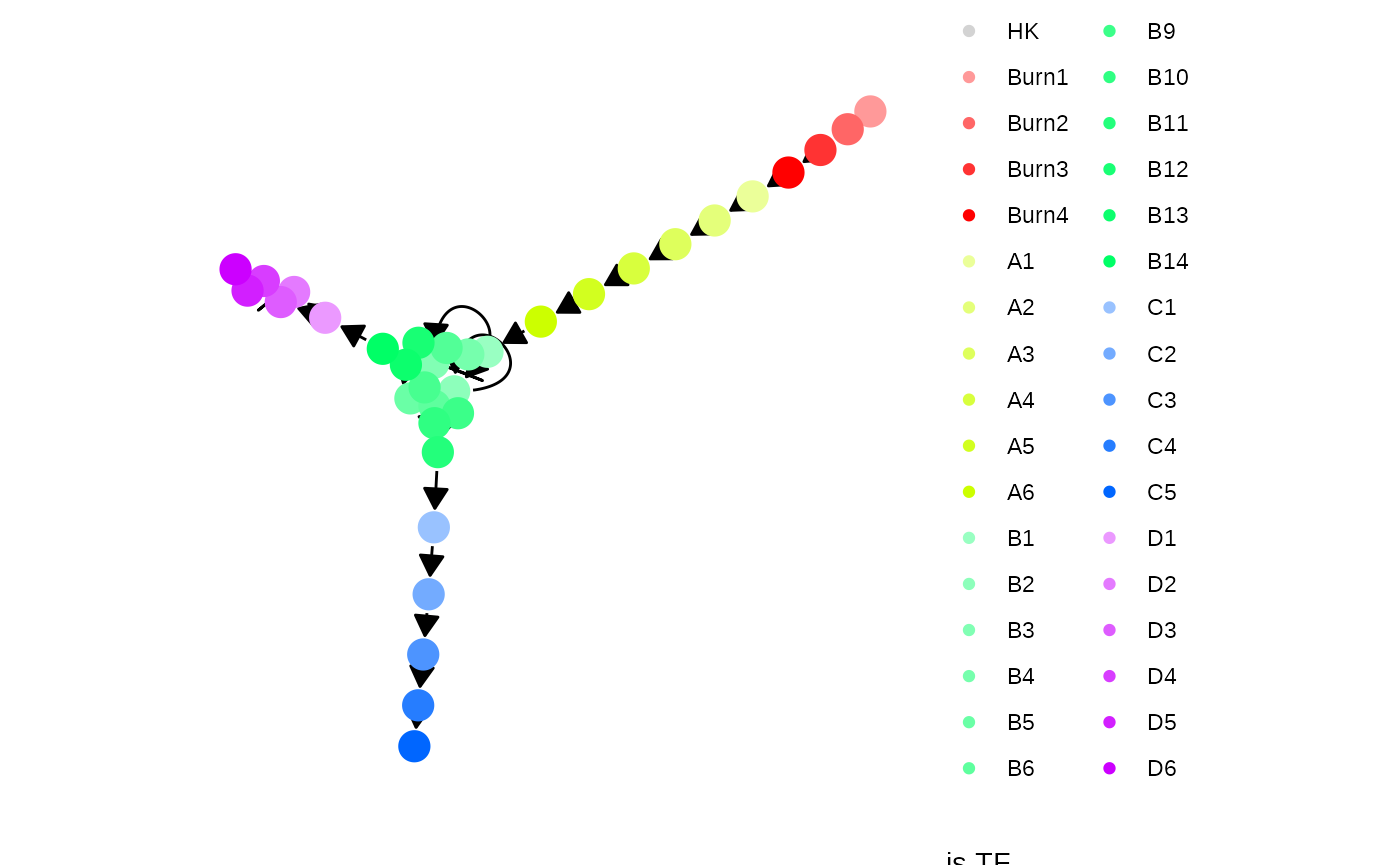
Step 3: Sample target genes and housekeeping genes (HKs)
Next, target genes and housekeeping genes are added to the network by sampling a gold standard gene regulatory network using the Page Rank algorithm. Target genes are regulated by TFs or other target genes, while HKs are only regulated by themselves.
model <- generate_feature_network(model)
plot_feature_network(model)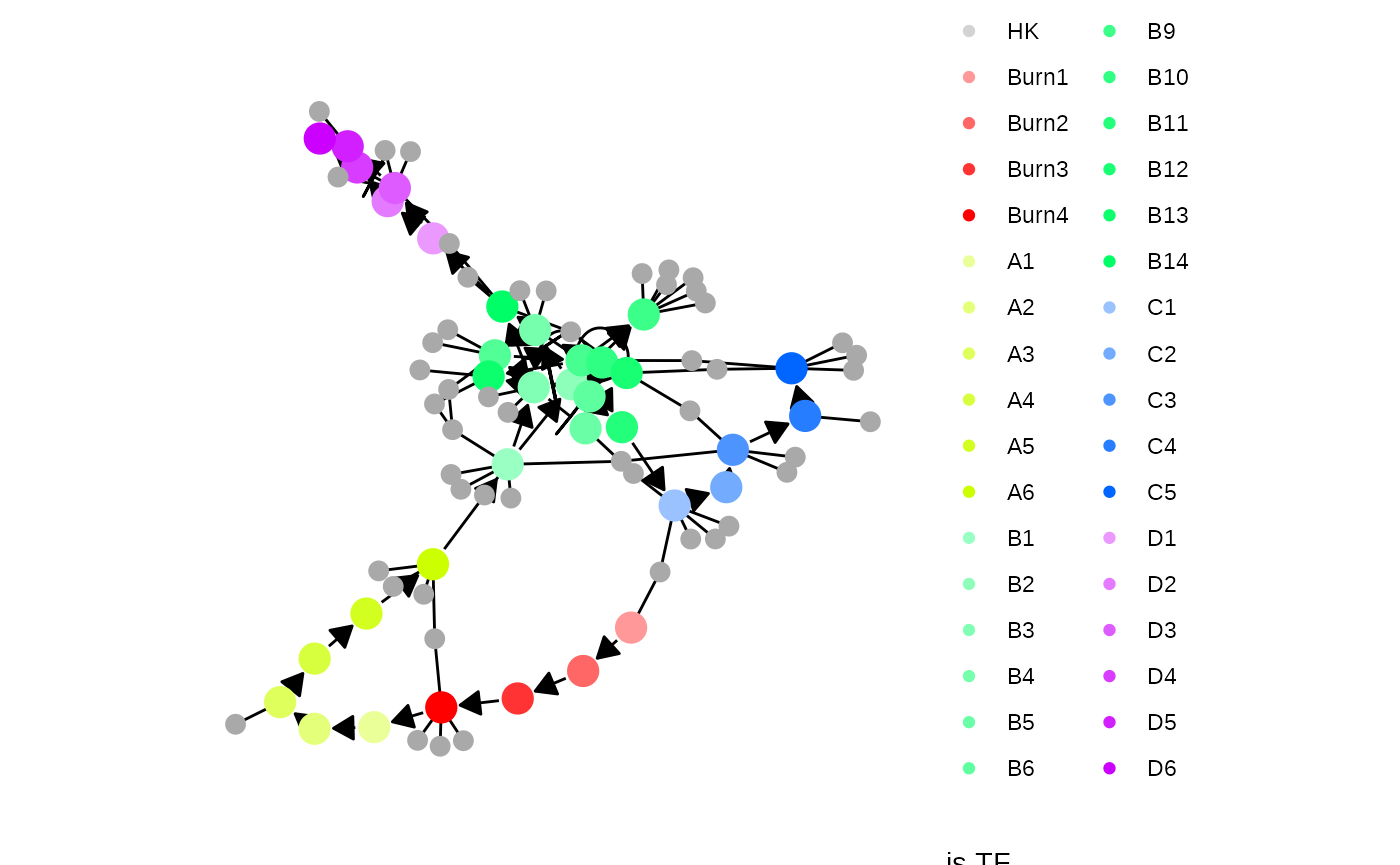
plot_feature_network(model, show_hks = TRUE)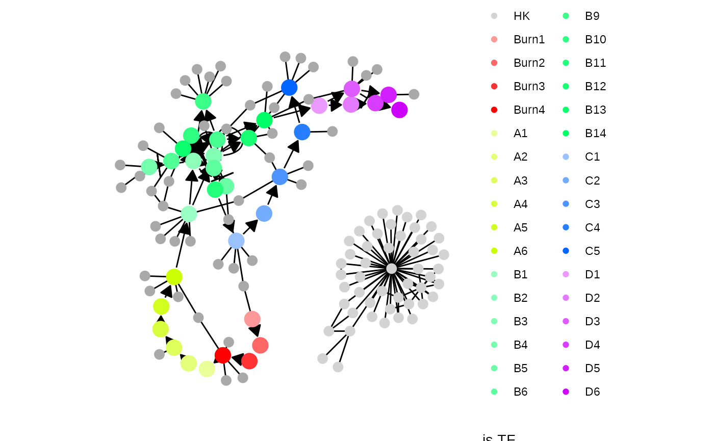
Step 4: Generate kinetics
Note that the target network does not show the effect of some interactions, because these are generated along with other kinetics parameters of the SSA simulation.
model <- generate_kinetics(model)
plot_feature_network(model)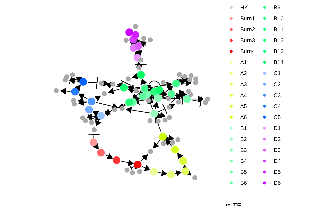
plot_feature_network(model, show_hks = TRUE)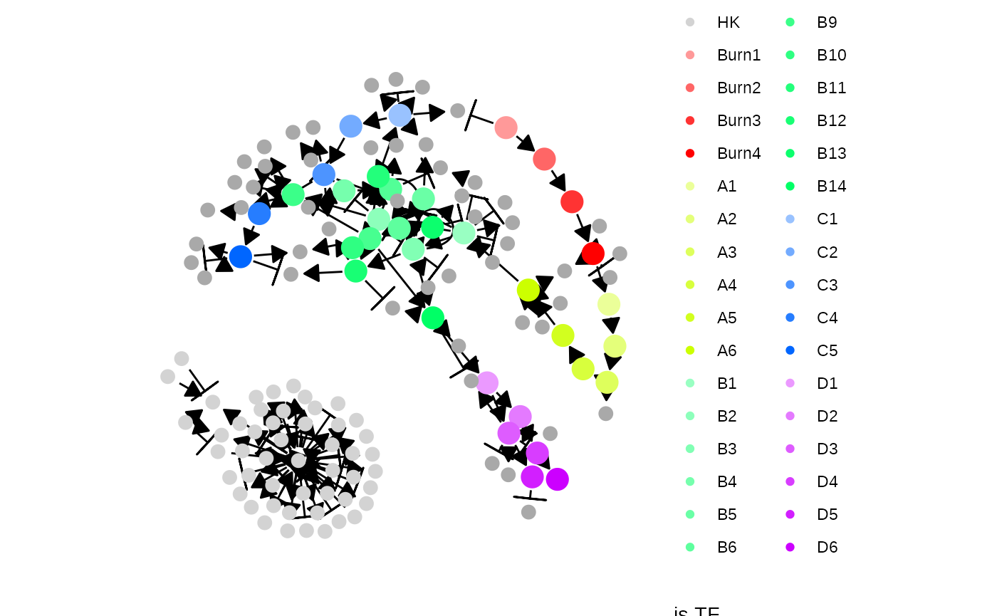
Step 5: Simulate gold standard
The gold standard is simulated by enabling certain parts of the module network and performing ODE simulations. The gold standard are visualised by performing a dimensionality reduction on the mRNA expression values.
model <- generate_gold_standard(model)
plot_gold_simulations(model) + scale_colour_brewer(palette = "Dark2")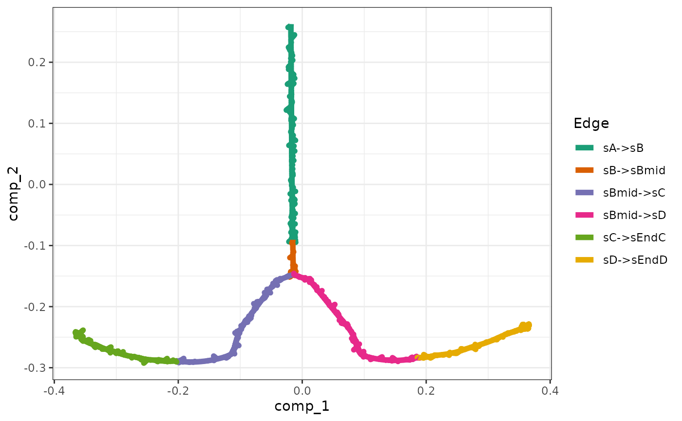
The expression of the modules (average of TFs) can be visualised as follows.
plot_gold_expression(model, what = "mol_mrna") # mrna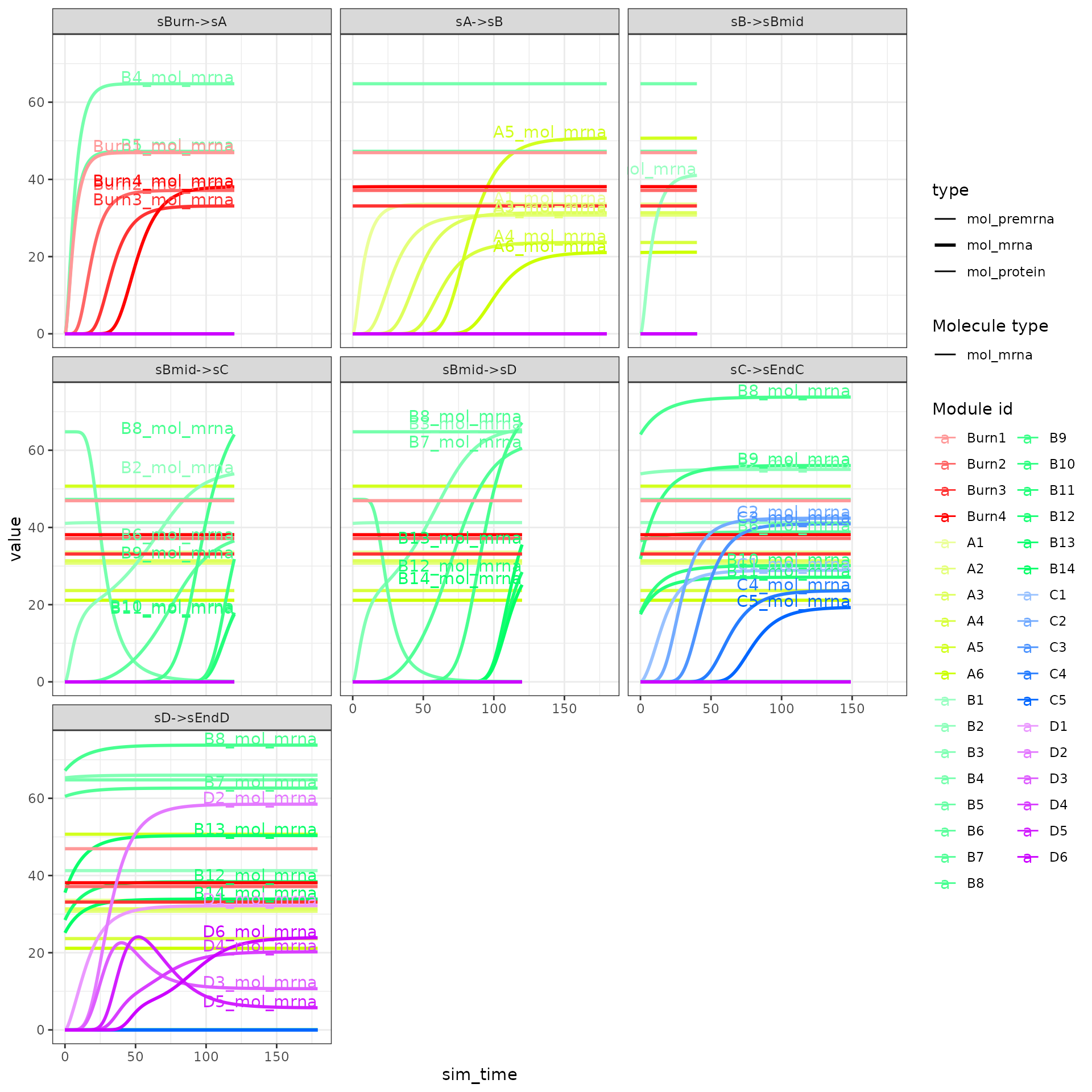
plot_gold_expression(model, label_changing = FALSE) # premrna, mrna, and protein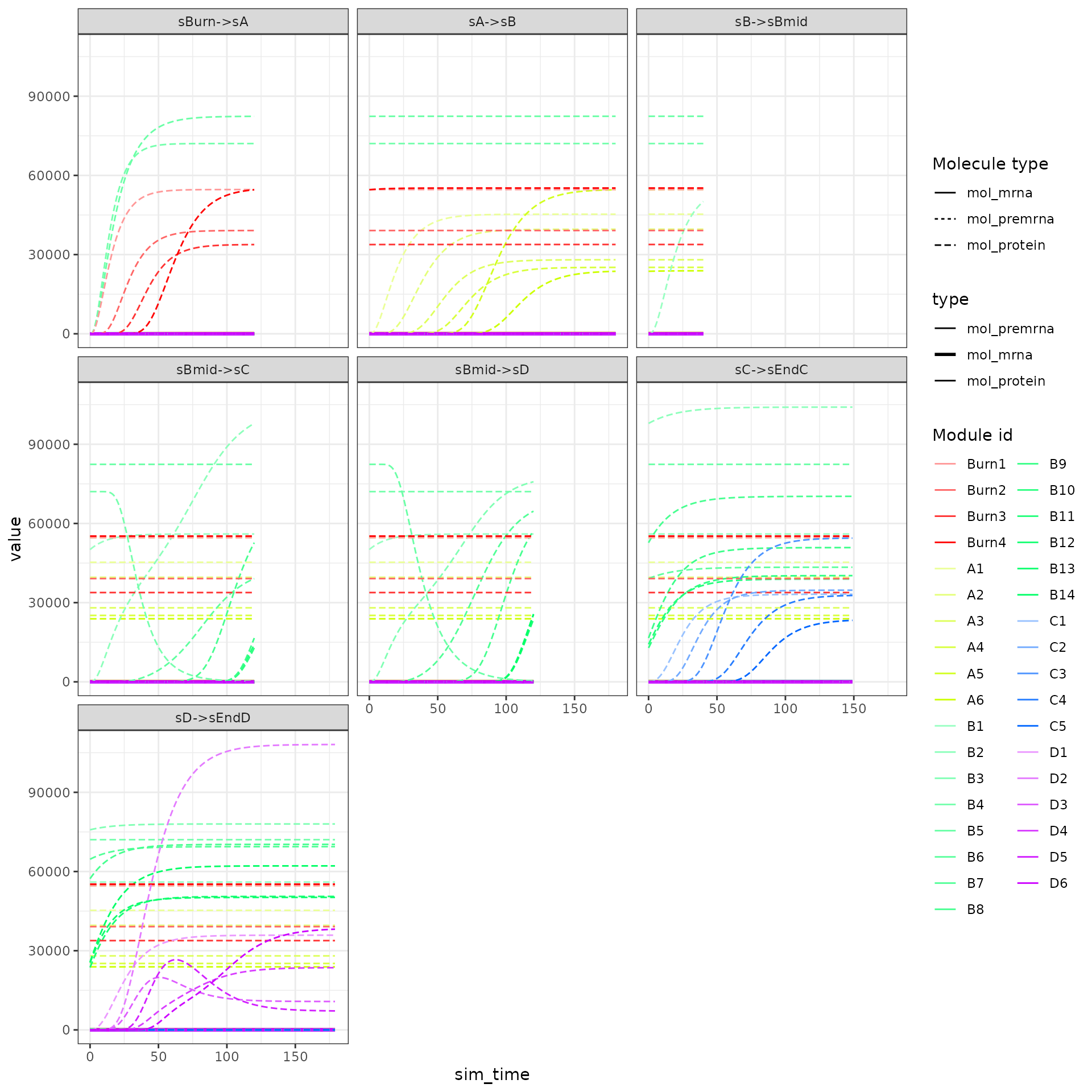
Step 6: Simulate cells.
Cells are simulated by running SSA simulations. The simulations are again using dimensionality reduction.
model <- generate_cells(model)
plot_simulations(model)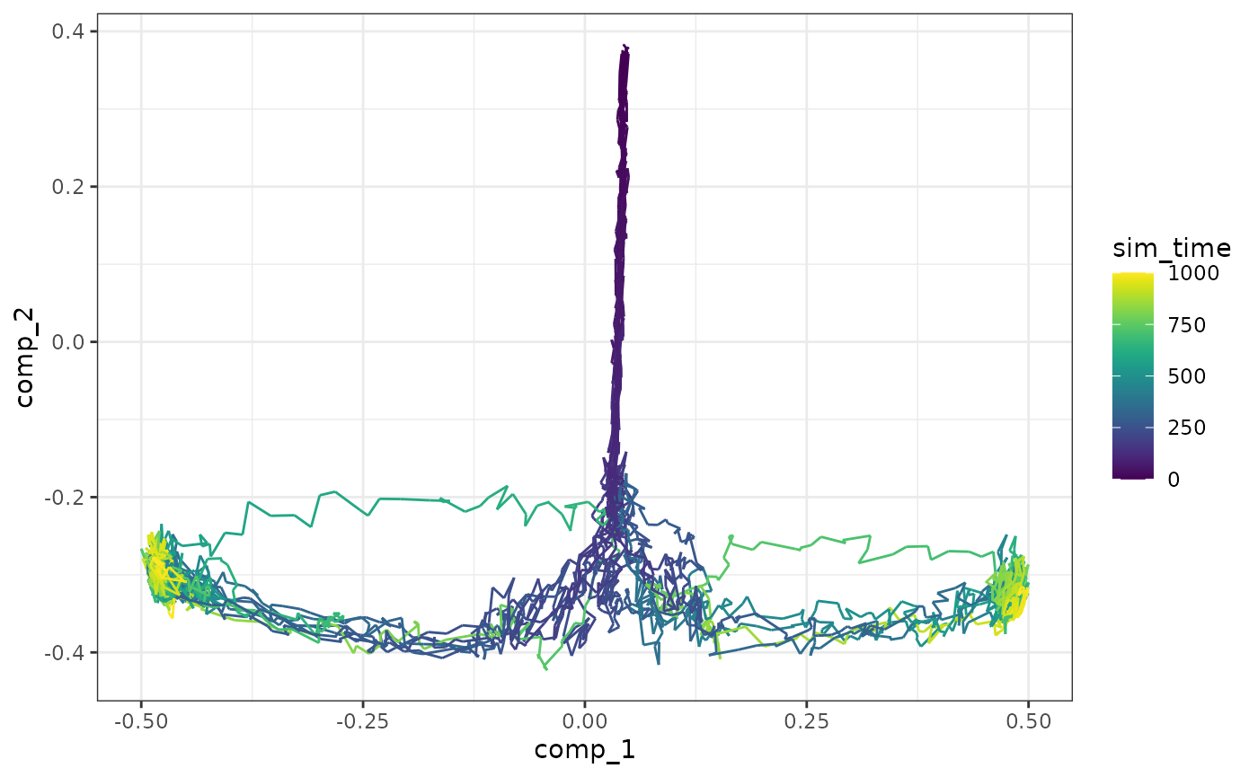
The gold standard can be overlayed on top of the simulations.
plot_gold_simulations(model) + scale_colour_brewer(palette = "Dark2")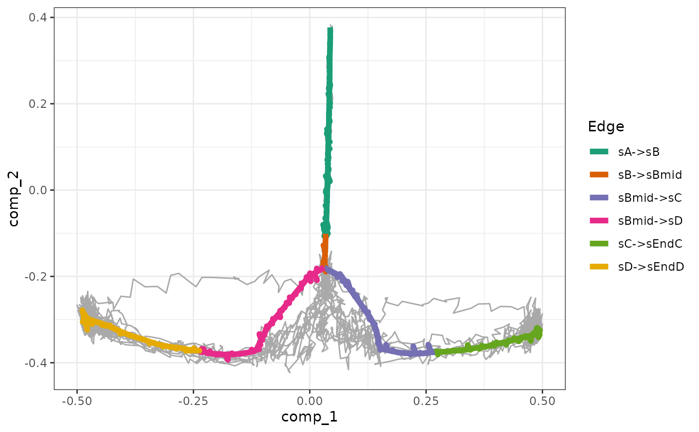
We can check how each segment of a simulation is mapped to the gold standard.
plot_gold_mappings(model, do_facet = FALSE) + scale_colour_brewer(palette = "Dark2")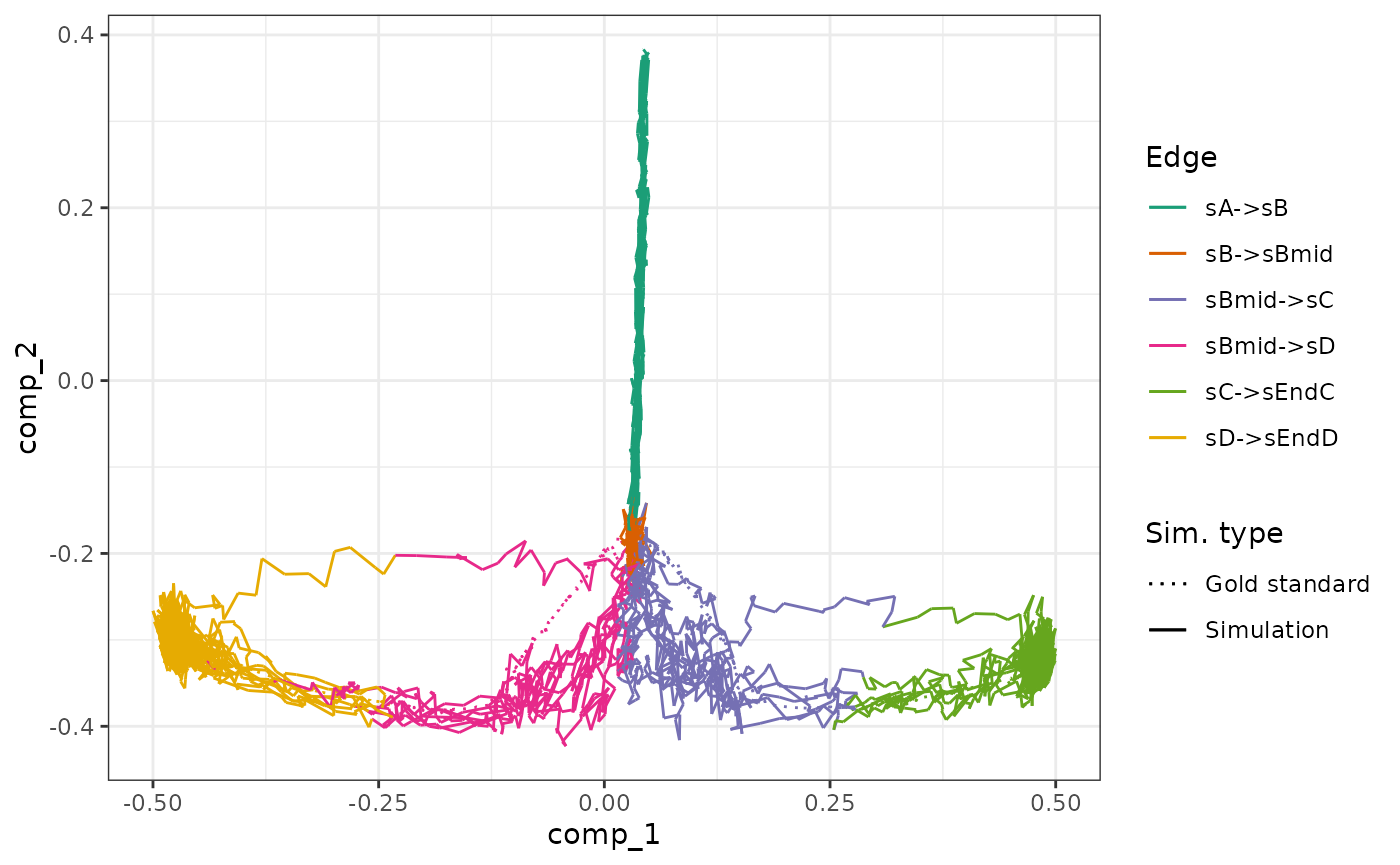
The expression of the modules (average of TFs) of a single simulation can be visualised as follows.
plot_simulation_expression(model, 1:4, what = "mol_mrna")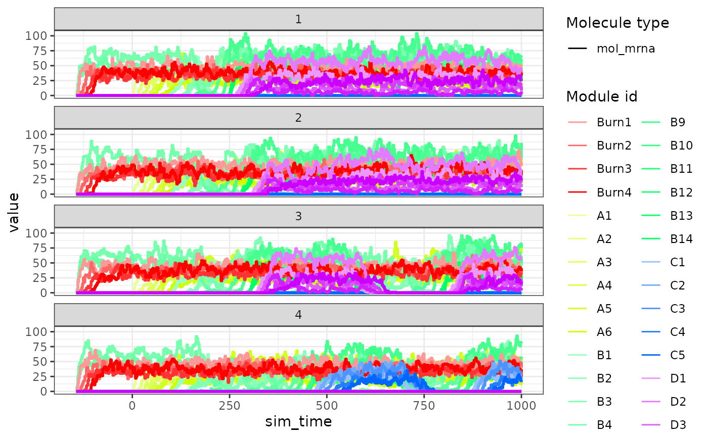
Step 7: Experiment emulation
Effects from performing a single-cell RNA-seq experiment can be emulated as follows.
model <- generate_experiment(model)Step 8: Convert to a dyno object
Converting the dyngen to a dyno object allows you to visualise the
dataset using the dynplot functions, or infer trajectories
using dynmethods.
dataset <- as_dyno(model)## Loading required namespace: dynwrapVisualise with dynplot
library(dynplot)
plot_dimred(dataset)
## Coloring by milestone## Using milestone_percentages from trajectory## Warning: Using `size` aesthetic for lines was deprecated in ggplot2 3.4.0.
## ℹ Please use `linewidth` instead.
## ℹ The deprecated feature was likely used in the dynplot package.
## Please report the issue at <https://github.com/dynverse/dynplot/issues>.
## This warning is displayed once per session.
## Call `lifecycle::last_lifecycle_warnings()` to see where this warning was
## generated.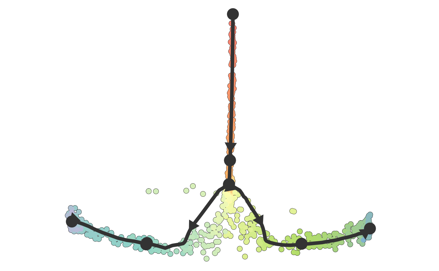
plot_graph(dataset)## Coloring by milestone
## Using milestone_percentages from trajectory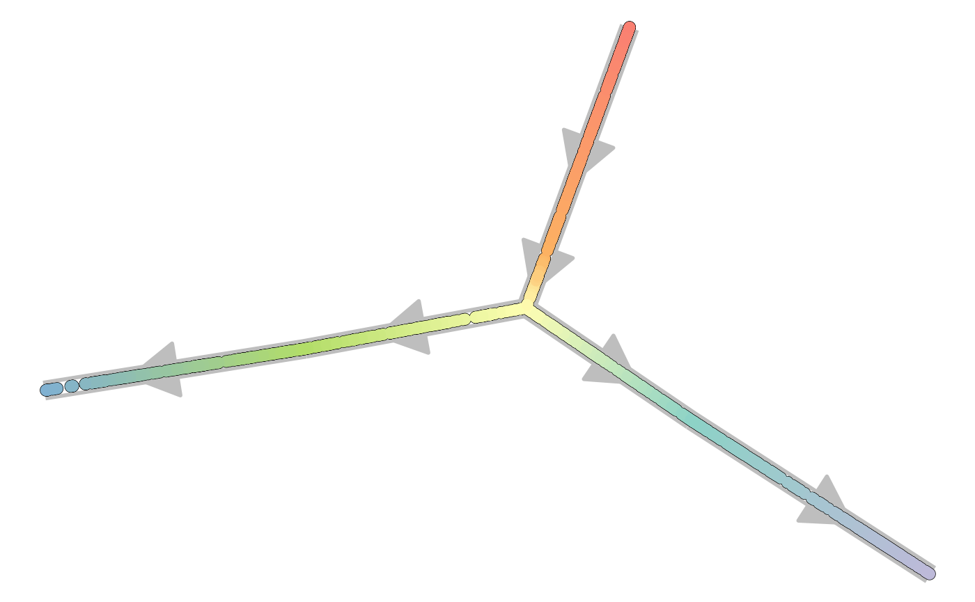
Step 8 alternative: Convert to an anndata/SCE/Seurat object
dyngen 1.0.0 allows converting the output to an anndata,
SCE or Seurat object as well. Check out the anndata
documentation on how to install anndata for R.
One-shot function
dyngen also provides a one-shot function for running all
of the steps all at once and producing plots.
out <- generate_dataset(
  config,
  format = "dyno",
  make_plots = TRUE
)
dataset <- out$dataset
model <- out$model
print(out$plot)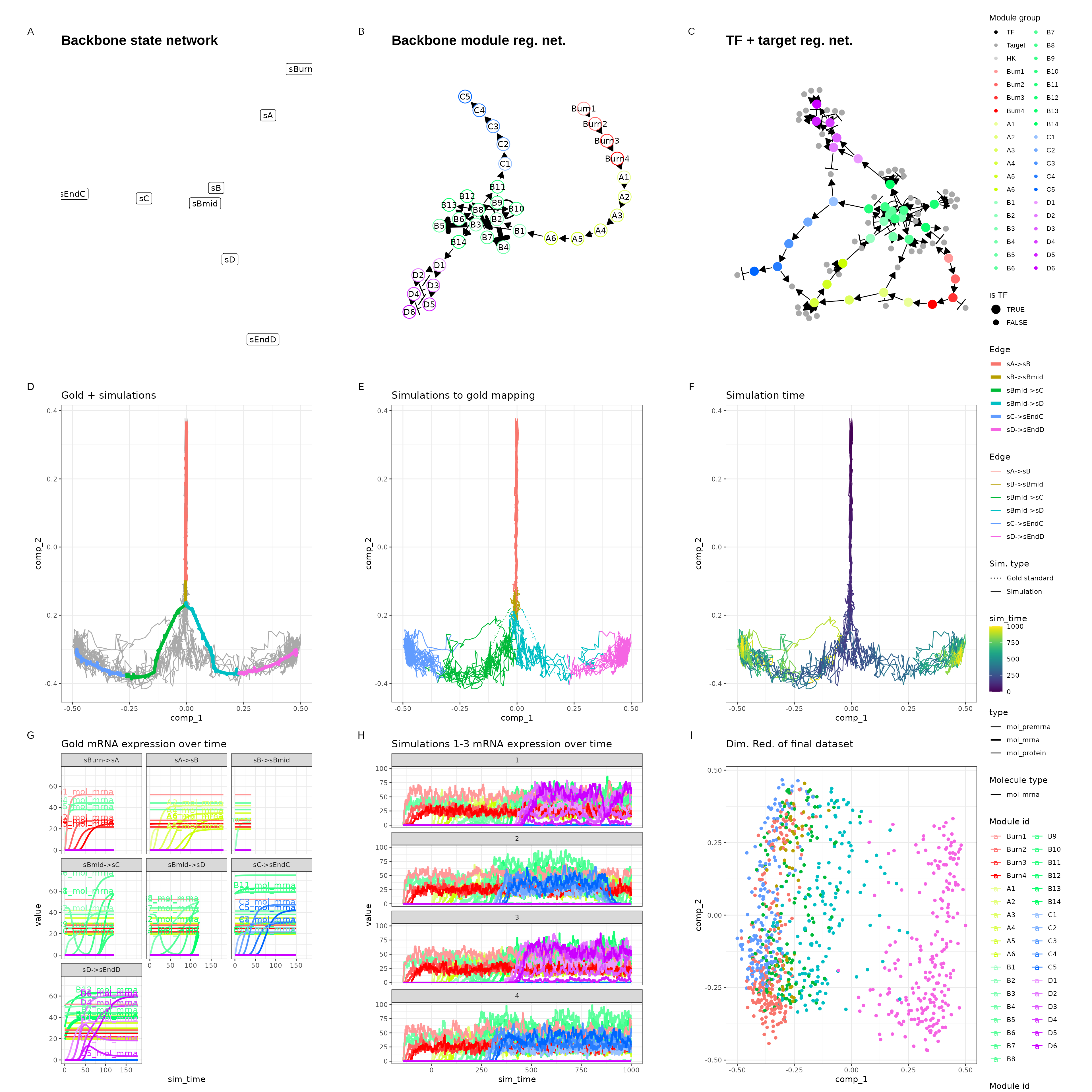
dataset and model can be used in much the
same way as before.
## Loading required package: dynfeature## Loading required package: dynguidelines## Loading required package: dynmethods## Loading required package: dynwrap
plot_dimred(dataset)## Coloring by milestone## Using milestone_percentages from trajectory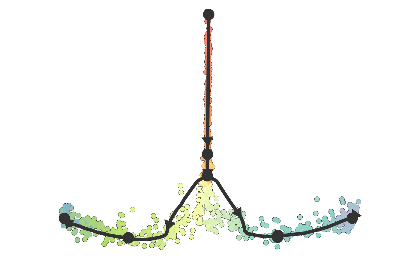
plot_graph(dataset)## Coloring by milestone
## Using milestone_percentages from trajectory