Advanced: Simulating a knockout experiment • dyngen

dyngen supports simulating knockout (or knockdown) experiments. In this experiment, dyngen is run twice (similar to the vignette on simulating batch effects), once for the wild type (WT), and once for the knockout (KO).

Initialising the experiment

First, create the ‘common’ part of the dyngen simulation as follows. This will ensure that the gene regulatory network-part of the simulation is exactly the same.

library(tidyverse)
library(dyngen)

set.seed(1)

backbone <- backbone_bifurcating()

config <-
  initialise_model(
    backbone = backbone,
    num_cells = 1000,
    num_tfs = nrow(backbone$module_info),
    num_targets = 250,
    num_hks = 250,
    simulation_params = simulation_default(
      census_interval = 10, 
      ssa_algorithm = ssa_etl(tau = 300 / 3600),
      experiment_params = simulation_type_wild_type(num_simulations = 100)
    )
  )

# the simulation is being sped up because rendering all vignettes with one core
# for pkgdown can otherwise take a very long time
set.seed(1)

config <-
  initialise_model(
    backbone = backbone,
    num_cells = 1000,
    num_tfs = nrow(backbone$module_info),
    num_targets = 50,
    num_hks = 50,
    verbose = interactive(),
    download_cache_dir = tools::R_user_dir("dyngen", "data"),
    simulation_params = simulation_default(
      census_interval = 5, 
      ssa_algorithm = ssa_etl(tau = 300/3600),
      experiment_params = simulation_type_wild_type(num_simulations = 10)
    )
  )

model_common <-
  config %>%
  generate_tf_network() %>%
  generate_feature_network() %>% 
  generate_kinetics() %>%
  generate_gold_standard()

Simulate wild type

Simulating the wild type is easy, as it is the standard dyngen way of simulating cells.

model_wt <- model_common %>%
  generate_cells()

plot_gold_mappings(model_wt, do_facet = FALSE)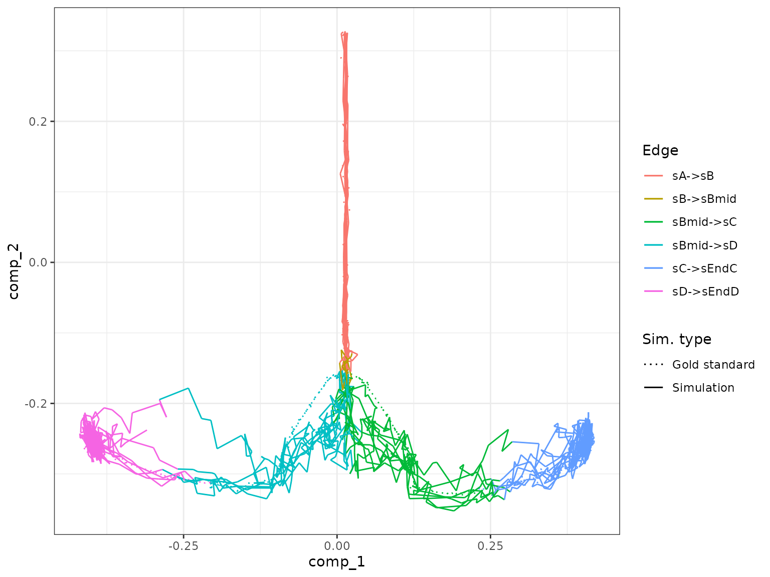

Simulate knockout

To simulate a gene knockout, the experiment type of the simulation is changed from wild type (see first code block) to knockdown. The simulation_type_knockdown() function is actually designed to perform single-cell knockdowns of 1 to 5 random genes, but this behaviour can be overridden by setting the following parameters:

genes: list of gene ids to be knocked out,
num_genes: number of genes to be knocked out per cell (sampled randomly),
multiplier: the fraction of transcription rate after KO (0 → no transcription, 1 → no KO).

In this case, looking at the module network of the bifurcation model it is possible to see that the B3 gene module is important for diversification of cells towards one particular cell lineage (to verify, one can draw out model_common$module_network on paper).

plot_backbone_modulenet(model_common)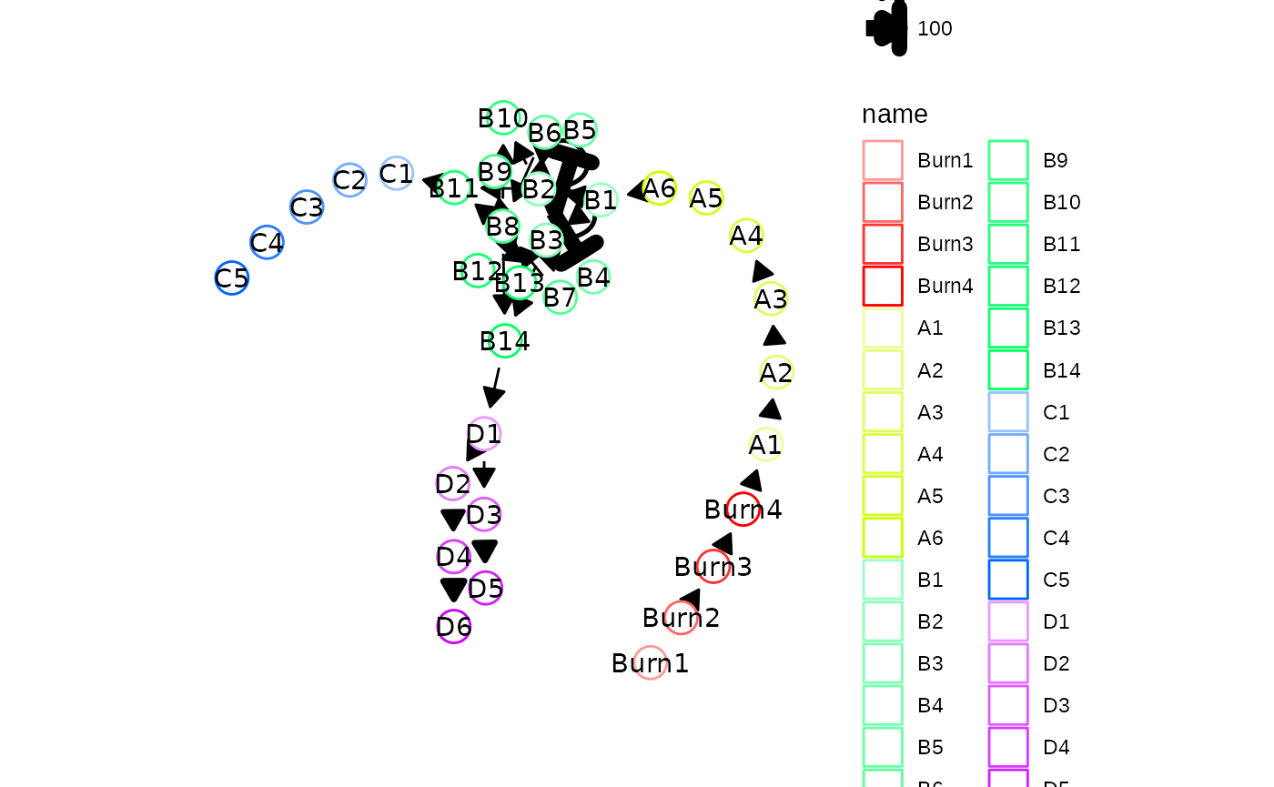

b3_genes <- model_common$feature_info %>% filter(module_id == "B3") %>% pull(feature_id)

By knocking out the gene "", one of the two branches will be inhibited.

model_ko <- model_common
model_ko$simulation_params$experiment_params <- simulation_type_knockdown(
  num_simulations = 100L,
  timepoint = 0, 
  genes = b3_genes,
  num_genes = length(b3_genes),
  multiplier = 0
)

Running the simulation will generate a warning stating that some of the gold standard edges were not covered by any of the simulations, but that’s to be expected since we knocked it out. We can see that indeed no simulation managed to enter the second branch (with end state D).

model_ko <- model_ko %>%
  generate_cells()

## Warning in .generate_cells_predict_state(model): Simulation does not contain all
## gold standard edges. This simulation likely suffers from bad kinetics; choose a
## different seed and rerun.

plot_gold_mappings(model_ko, do_facet = FALSE)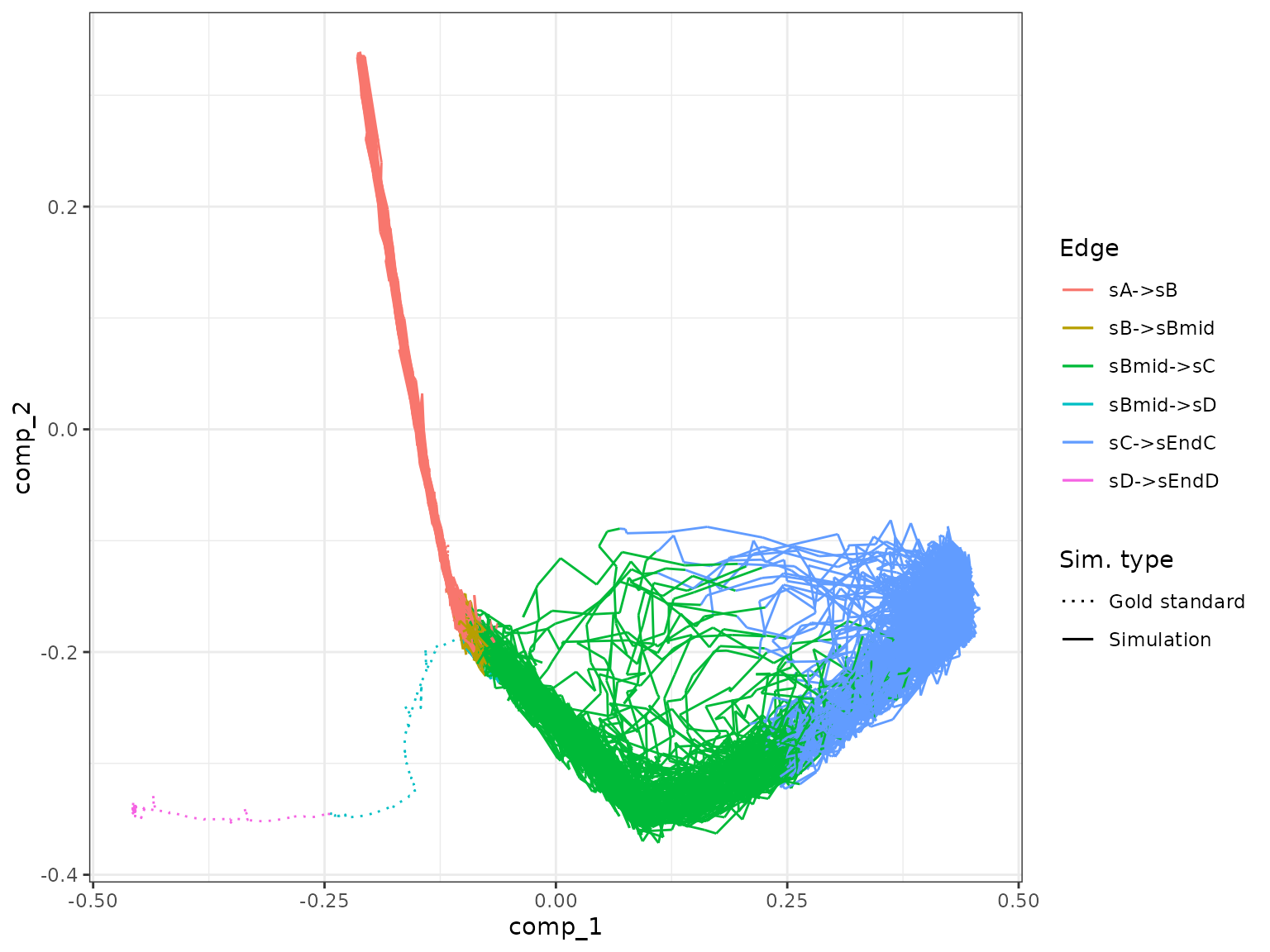

Combine outputs and visualise

We can combine both simulations into one simulation and visualise the output.

model_comb <-
  combine_models(list(WT = model_wt, KO = model_ko)) %>% 
  generate_experiment()

## Warning in params$fun(network = network, sim_meta = sim_meta, params = model$experiment_params, : Certain backbone segments are not covered by any of the simulations. If this is intentional, please ignore this warning.
##   Otherwise, increase the number of simulations (see `?simulation_default`) or decreasing the census interval (see `?simulation_default`).

## Warning in params$fun(network = network, sim_meta = sim_meta, params = model$experiment_params, : One of the branches did not obtain enough simulation steps.
##   Increase the number of simulations (see `?simulation_default`) or decreasing the census interval (see `?simulation_default`).

plot_simulations(model_comb)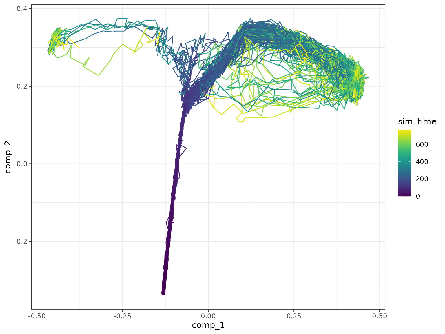

plot_gold_mappings(model_comb, do_facet = FALSE)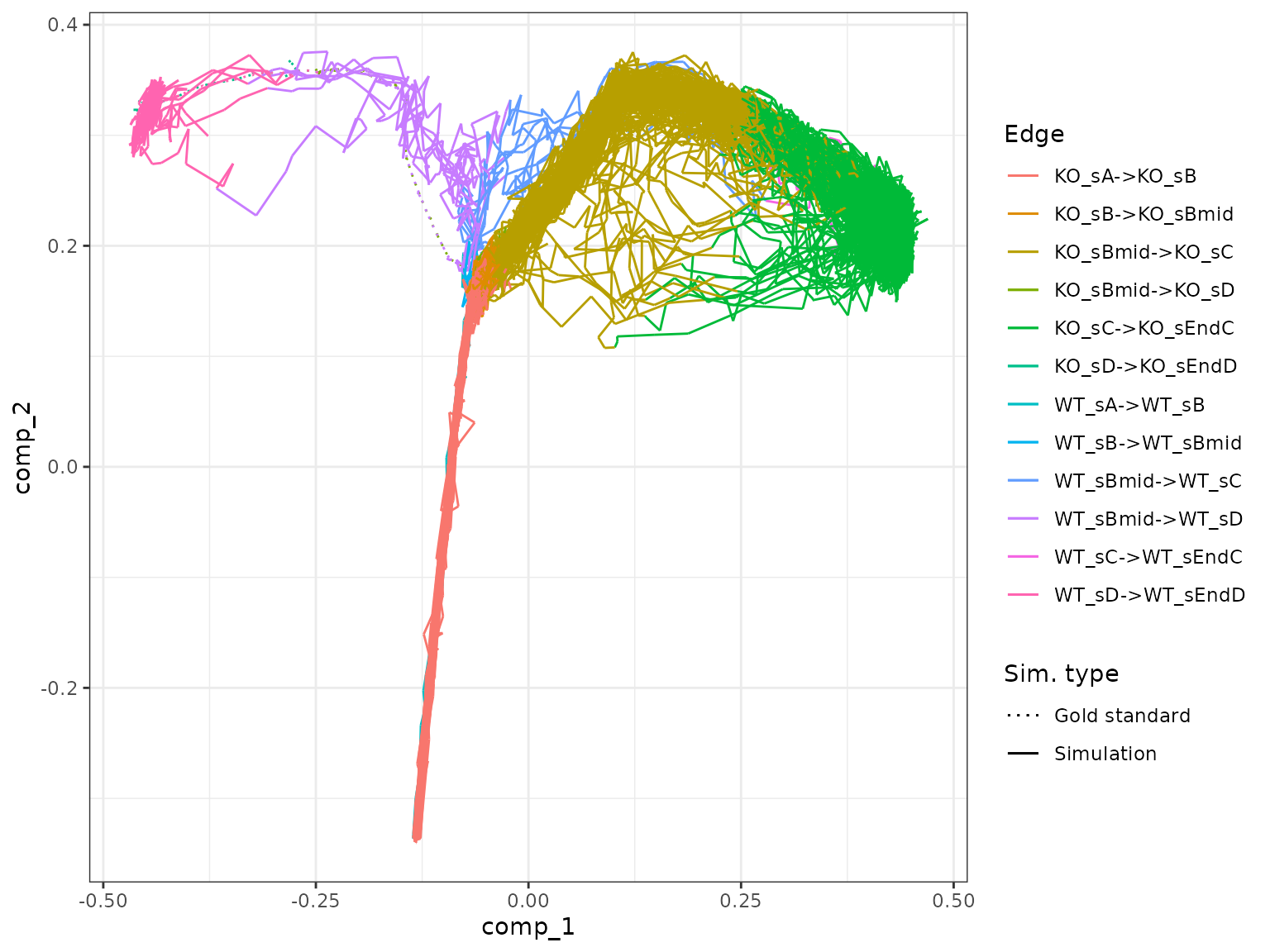

Visualise the dataset using dyno.

library(dyno)

## Loading required package: dynfeature

## Loading required package: dynguidelines

## Loading required package: dynmethods

## Loading required package: dynplot

## Loading required package: dynwrap

dataset <- as_dyno(model_comb)
plot_dimred(dataset)

## Coloring by milestone

## Using milestone_percentages from trajectory

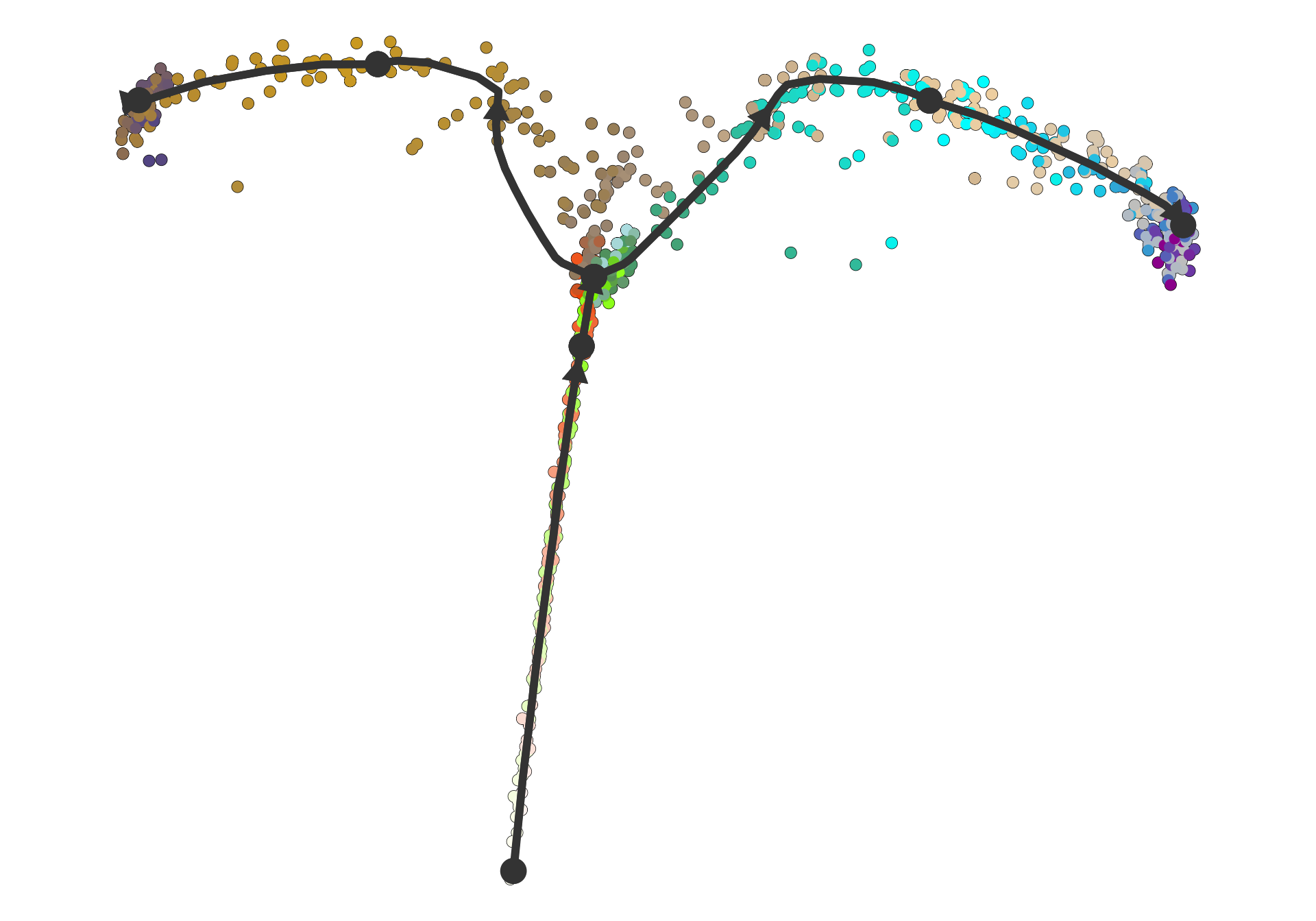
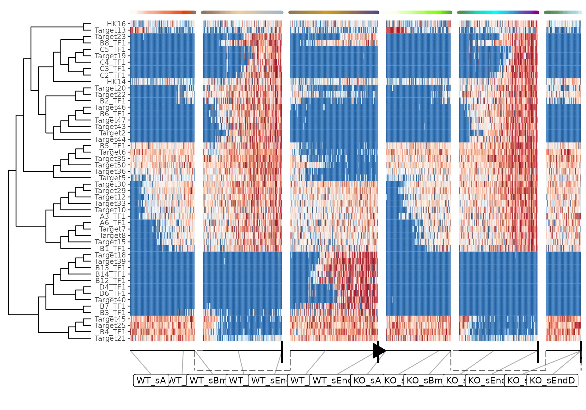
plot_heatmap(dataset, features_oi = 50)

## No features of interest provided, selecting the top 50 features automatically

## Using dynfeature for selecting the top 50 features

## root cell or milestone not provided, trying first outgoing milestone_id

## Using 'WT_sA' as root

## Coloring by milestone