Advanced: Constructing a custom backbone

You may want to construct your own custom backbone as opposed to those predefined in dyngen in order to obtain a desired effect. You can do so in one of two ways.

Backbone lego

You can use the bblego functions in order to create custom backbones using so-called ‘backbone lego blocks’. Please note that bblego only allows you to create tree-shaped backbones (so no cycles), but in 90% of cases will be exactly what you need and in the remaining 10% of cases these functions will still get you 80% of where you need to be.

Here is an example of a bifurcating trajectory.

library(dyngen)
library(tidyverse)

set.seed(1)

backbone <- bblego(
  bblego_start("A", type = "simple", num_modules = 2),
  bblego_linear("A", "B", type = "simple", num_modules = 4),
  bblego_branching("B", c("C", "D"), type = "simple"),
  bblego_end("C", type = "doublerep2", num_modules = 4),
  bblego_end("D", type = "doublerep1", num_modules = 7)
)

config <- 
  initialise_model(
    backbone = backbone,
    num_tfs = nrow(backbone$module_info),
    num_targets = 500,
    num_hks = 500,
    verbose = FALSE
  )

# the simulation is being sped up because rendering all vignettes with one core
# for pkgdown can otherwise take a very long time
config <- 
  initialise_model(
    backbone = backbone,
    num_tfs = nrow(backbone$module_info),
    num_targets = 50,
    num_hks = 50,
    verbose = interactive(),
    simulation_params = simulation_default(
      ssa_algorithm = ssa_etl(tau = .01),
      census_interval = 1,
      experiment_params = simulation_type_wild_type(num_simulations = 10)
    ),
    download_cache_dir = tools::R_user_dir("dyngen", "data")
  )

out <- generate_dataset(config, make_plots = TRUE)

print(out$plot)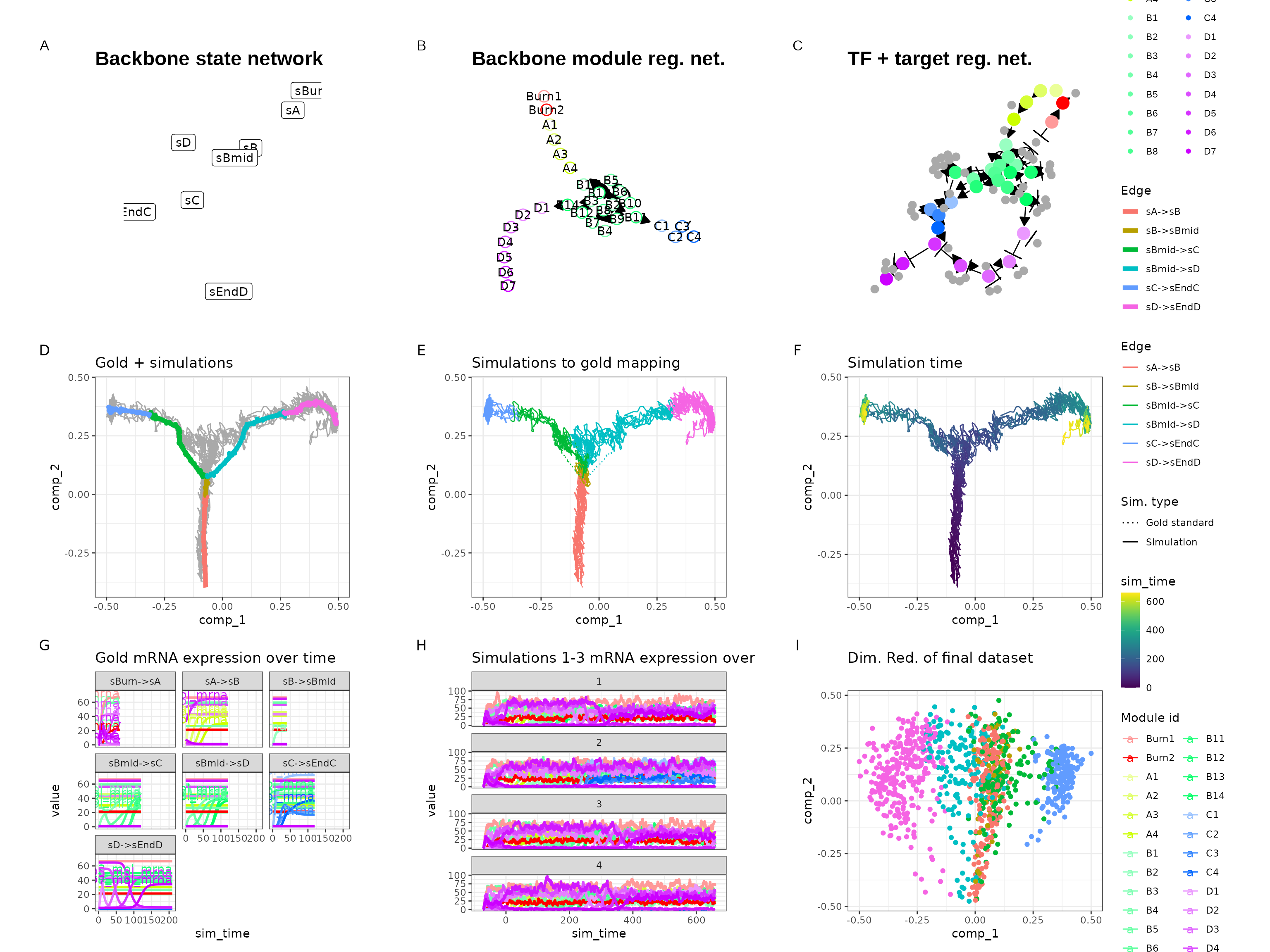

Check the following predefined backbones for some examples.

• backbone_bifurcating
• backbone_branching
• backbone_linear

Manually constructing backbone data frames

To get the most control over how a dyngen simulation is performed, you can construct a backbone manually (see ?backbone for the full spec). This is the only way to create some of the more specific backbone shapes such as disconnected, cyclic and converging.

This is an example of what data structures a backbone consists of.

Module info

A tibble containing meta information on the modules themselves. A module is a group of genes which, to some extent, shows the same expression behaviour. Several modules are connected together such that one or more genes from one module will regulate the expression of another module. By creating chains of modules, a dynamic behaviour in gene regulation can be created.

• module_id (character): the name of the module
• basal (numeric): basal expression level of genes in this module, must be between [0, 1]
• burn (logical): whether or not outgoing edges of this module will be active during the burn in phase
• independence (numeric): the independence factor between regulators of this module, must be between [0, 1]

module_info <- tribble(
  ~module_id, ~basal, ~burn, ~independence,
  "A1", 1, TRUE, 1,
  "A2", 0, TRUE, 1,
  "A3", 1, TRUE, 1,
  "B1", 0, FALSE, 1,
  "B2", 1, TRUE, 1,
  "C1", 0, FALSE, 1,
  "C2", 0, FALSE, 1,
  "C3", 0, FALSE, 1,
  "D1", 0, FALSE, 1,
  "D2", 0, FALSE, 1,
  "D3", 1, TRUE, 1,
  "D4", 0, FALSE, 1,
  "D5", 0, FALSE, 1
)

Module network

A tibble describing which modules regulate which other modules.

• from (character): the regulating module
• to (character): the target module
• effect (integer): 1L if the regulating module upregulates the target module, -1L if it downregulates
• strength (numeric): the strength of the interaction
• hill (numeric): hill coefficient, larger than 1 for positive cooperativity, between 0 and 1 for negative cooperativity

module_network <- tribble(
  ~from, ~to, ~effect, ~strength, ~hill,
  "A1", "A2", 1L, 10, 2,
  "A2", "A3", -1L, 10, 2,
  "A2", "B1", 1L, 1, 2,
  "B1", "B2", -1L, 10, 2,
  "B1", "C1", 1L, 1, 2,
  "B1", "D1", 1L, 1, 2,
  "C1", "C1", 1L, 10, 2,
  "C1", "D1", -1L, 100, 2,
  "C1", "C2", 1L, 1, 2,
  "C2", "C3", 1L, 1, 2,
  "C2", "A2", -1L, 10, 2,
  "C2", "B1", -1L, 10, 2,
  "C3", "A1", -1L, 10, 2,
  "C3", "C1", -1L, 10, 2,
  "C3", "D1", -1L, 10, 2,
  "D1", "D1", 1L, 10, 2,
  "D1", "C1", -1L, 100, 2,
  "D1", "D2", 1L, 1, 2,
  "D1", "D3", -1L, 10, 2,
  "D2", "D4", 1L, 1, 2,
  "D4", "D5", 1L, 1, 2,
  "D3", "D5", -1L, 10, 2
)

Expression patterns

A tibble describing the expected expression pattern changes when a cell is simulated by dyngen. Each row represents one transition between two cell states.

• from (character): name of a cell state
• to (character): name of a cell state
• module_progression (character): differences in module expression between the two states. Example: “+4,-1|+9|-4” means the expression of module 4 will go up at the same time as module 1 goes down; afterwards module 9 expression will go up, and afterwards module 4 expression will go down again.
• start (logical): Whether or not this from cell state is the start of the trajectory
• burn (logical): Whether these cell states are part of the burn in phase. Cells will not get sampled from these cell states.
• time (numeric): The duration of an transition.

expression_patterns <- tribble(
  ~from, ~to, ~module_progression, ~start, ~burn, ~time,
  "sBurn", "sA", "+A1,+A2,+A3,+B2,+D3", TRUE, TRUE, 60,
  "sA", "sB", "+B1", FALSE, FALSE, 60,
  "sB", "sC", "+C1,+C2|-A2,-B1,+C3|-C1,-D1,-D2", FALSE, FALSE, 80,
  "sB", "sD", "+D1,+D2,+D4,+D5", FALSE, FALSE, 120,
  "sC", "sA", "+A1,+A2", FALSE, FALSE, 60
)

Visualising the backbone

By wrapping these data structures as a backbone object, we can now visualise the topology of the backbone. Drawing the backbone module network by hand on a piece of paper can help you understand how the gene regulatory network works.

backbone <- backbone(
  module_info = module_info,
  module_network = module_network,
  expression_patterns = expression_patterns
)

config <- initialise_model(
  backbone = backbone,
  num_tfs = nrow(backbone$module_info),
  num_targets = 500,
  num_hks = 500,
  simulation_params = simulation_default(
    experiment_params = simulation_type_wild_type(num_simulations = 100),
    total_time = 600
  ),
  verbose = FALSE
)

plot_backbone_modulenet(config)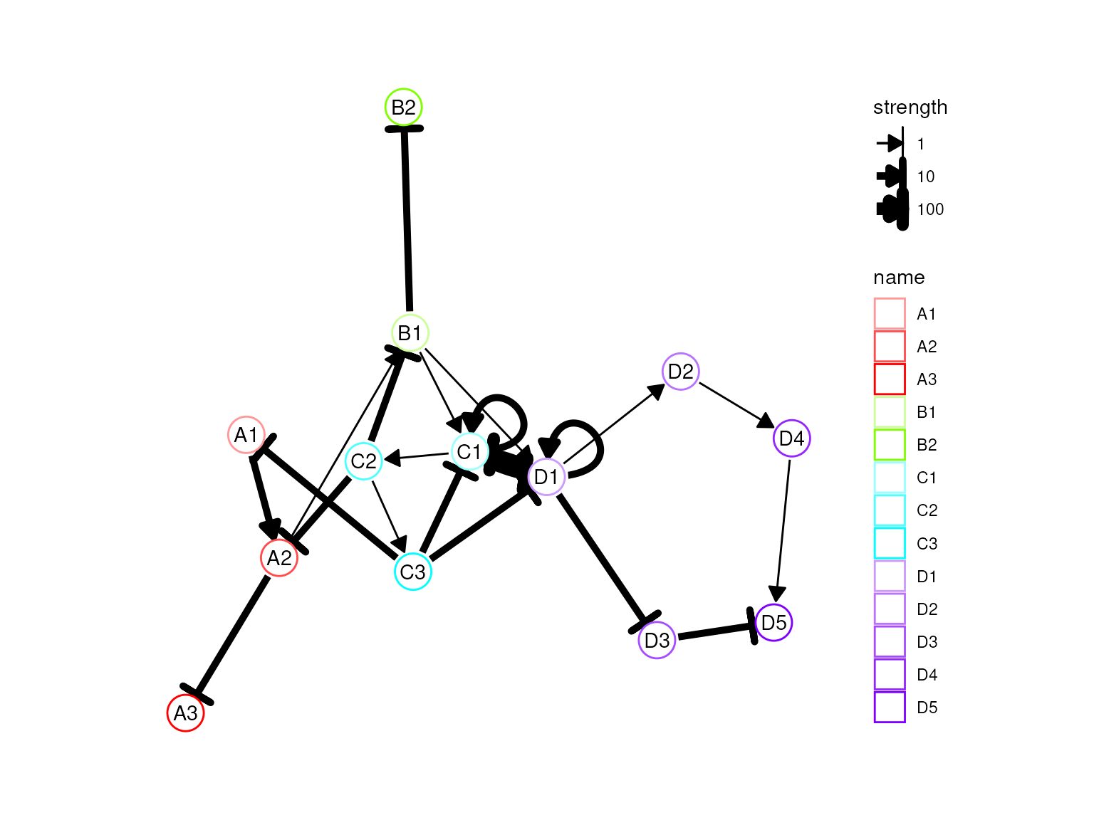

plot_backbone_statenet(config)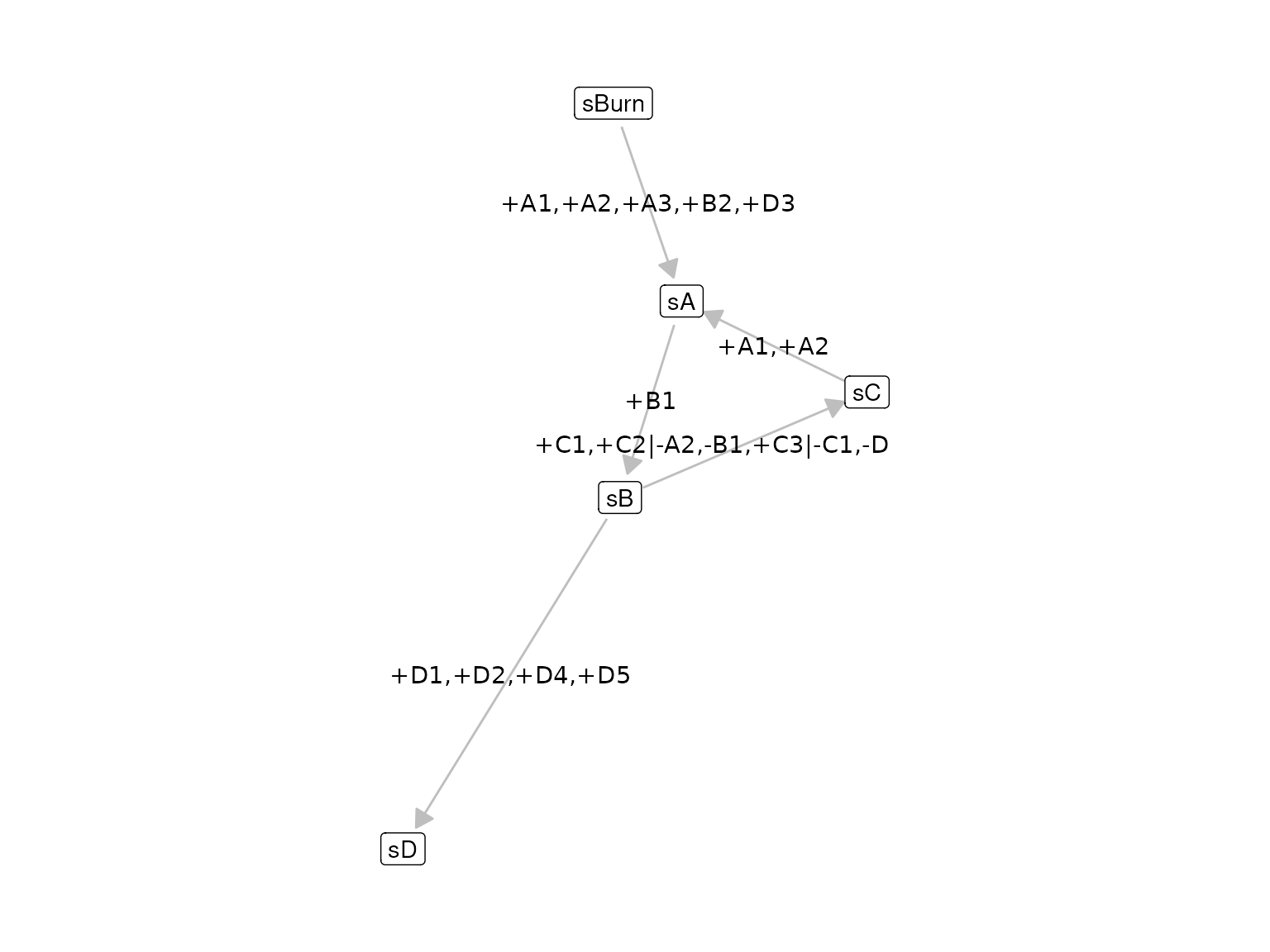

# the simulation is being sped up because rendering all vignettes with one core
# for pkgdown can otherwise take a very long time
config <- 
  initialise_model(
    backbone = backbone,
    num_tfs = nrow(backbone$module_info),
    num_targets = 50,
    num_hks = 50,
    verbose = interactive(),
    simulation_params = simulation_default(
      ssa_algorithm = ssa_etl(tau = .01),
      census_interval = 2,
      experiment_params = simulation_type_wild_type(num_simulations = 20),
      total_time = 600
    ),
    download_cache_dir = tools::R_user_dir("dyngen", "data")
  )

Simulation

This allows you to simulate the following dataset.

out <- generate_dataset(config, make_plots = TRUE)

## Warning in params$fun(network = network, sim_meta = sim_meta, params = model$experiment_params, : One of the branches did not obtain enough simulation steps.
##   Increase the number of simulations (see `?simulation_default`) or decreasing the census interval (see `?simulation_default`).

print(out$plot)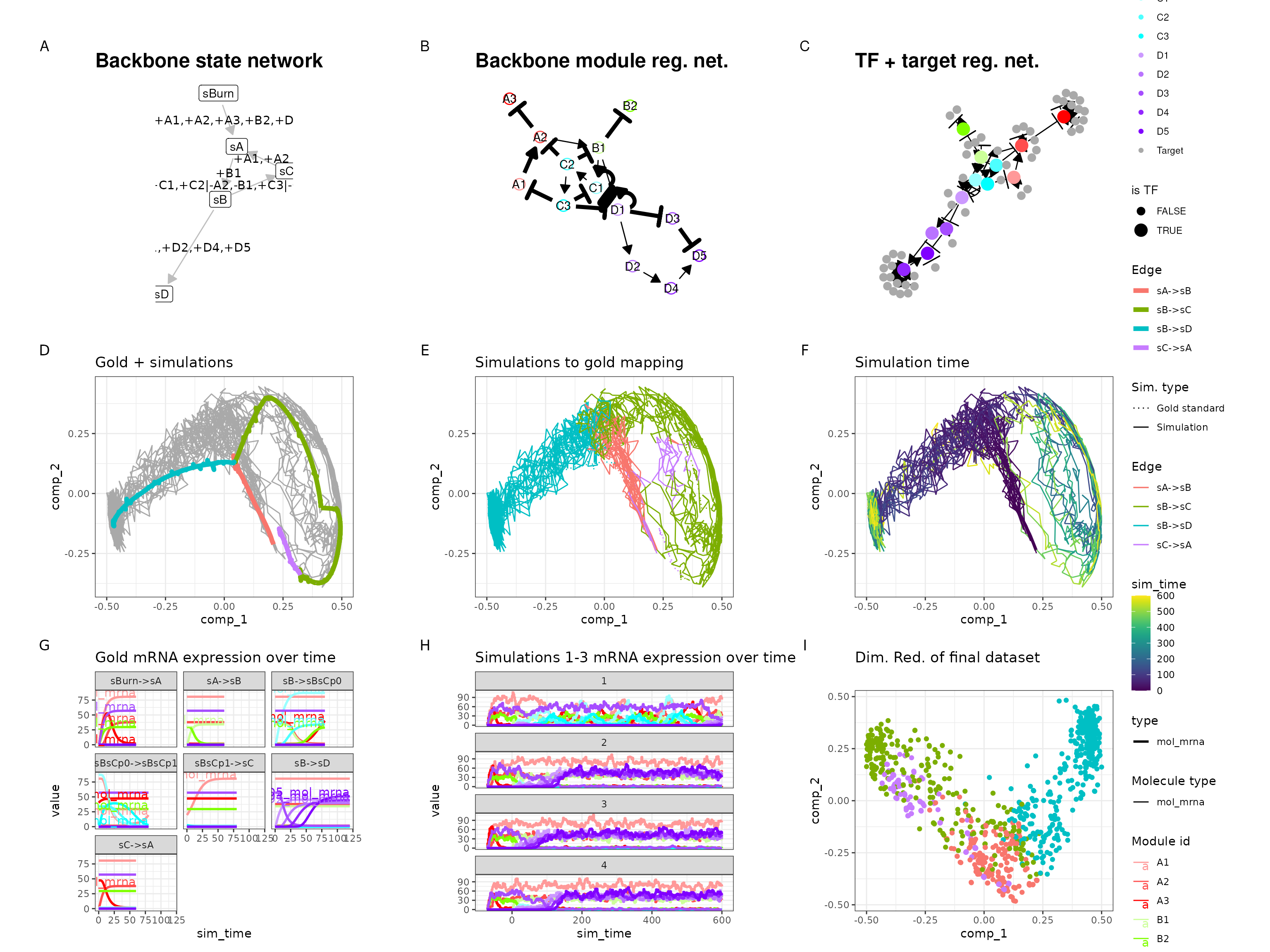

More information

dyngen has a lot of predefined backbones. The following predefined backbones construct the backbone manually (as opposed to using bblego).

• backbone_bifurcating_converging
• backbone_bifurcating_cycle
• backbone_bifurcating_loop
• backbone_binary_tree
• backbone_consecutive_bifurcating
• backbone_converging
• backbone_cycle
• backbone_cycle_simple
• backbone_disconnected
• backbone_linear_simple
• backbone_trifurcating

Combination of bblego and manual

You can also use parts of the ‘bblego’ framework to construct a backbone manually. That’s because the bblego functions simply generate the three data frames (module_info, module_network and expression_patterns) required to construct a backbone manually. For example:

part0 <- bblego_start("A", type = "simple", num_modules = 2)
part1 <- bblego_linear("A", "B", type = "simple", num_modules = 3)
part3 <- bblego_end("C", type = "simple", num_modules = 3)
part4 <- bblego_end("D", type = "simple", num_modules = 3)

part1

## $module_info
## # A tibble: 3 × 4
##   module_id basal burn  independence
##   <chr>     <dbl> <lgl>        <dbl>
## 1 A1            0 FALSE            1
## 2 A2            0 FALSE            1
## 3 A3            0 FALSE            1
## 
## $module_network
## # A tibble: 3 × 5
##   from  to    effect strength  hill
##   <chr> <chr>  <int>    <dbl> <dbl>
## 1 A1    A2         1        1     2
## 2 A2    A3         1        1     2
## 3 A3    B1         1        1     2
## 
## $expression_patterns
## # A tibble: 1 × 6
##   from  to    module_progression start burn   time
##   <chr> <chr> <chr>              <lgl> <lgl> <dbl>
## 1 sA    sB    +A1,+A2,+A3        FALSE FALSE    90

You can combine these components with a custom bifurcation component which can switch back and forth between end states.

part2 <- list(
  module_info = tribble(
    ~module_id, ~basal, ~burn, ~independence,
    "B1", 0, FALSE, 1,
    "B2", 0, FALSE, 1,
    "B3", 0, FALSE, 1
  ),
  module_network = tribble(
    ~from, ~to, ~effect, ~strength, ~hill,
    "B1", "B2", 1L, 1, 2,
    "B1", "B3", 1L, 1, 2,
    "B2", "B3", -1L, 3, 2,
    "B3", "B2", -1L, 3, 2,
    "B2", "C1", 1L, 1, 2,
    "B3", "D1", 1L, 1, 2
  ),
  expression_patterns = tribble(
    ~from, ~to, ~module_progression, ~start, ~burn, ~time,
    "sB", "sBmid", "+B1", FALSE, FALSE, 40,
    "sBmid", "sC", "+B2", FALSE, FALSE, 40,
    "sBmid", "sD", "+B3", FALSE, FALSE, 30
  )
)

backbone <- bblego(
  part0,
  part1,
  part2,
  part3,
  part4
)

config <- initialise_model(
  backbone = backbone,
  num_tfs = nrow(backbone$module_info),
  num_targets = 500,
  num_hks = 500,
  simulation_params = simulation_default(
    total_time = simtime_from_backbone(backbone) * 2
  ),
  verbose = FALSE
)

plot_backbone_modulenet(config)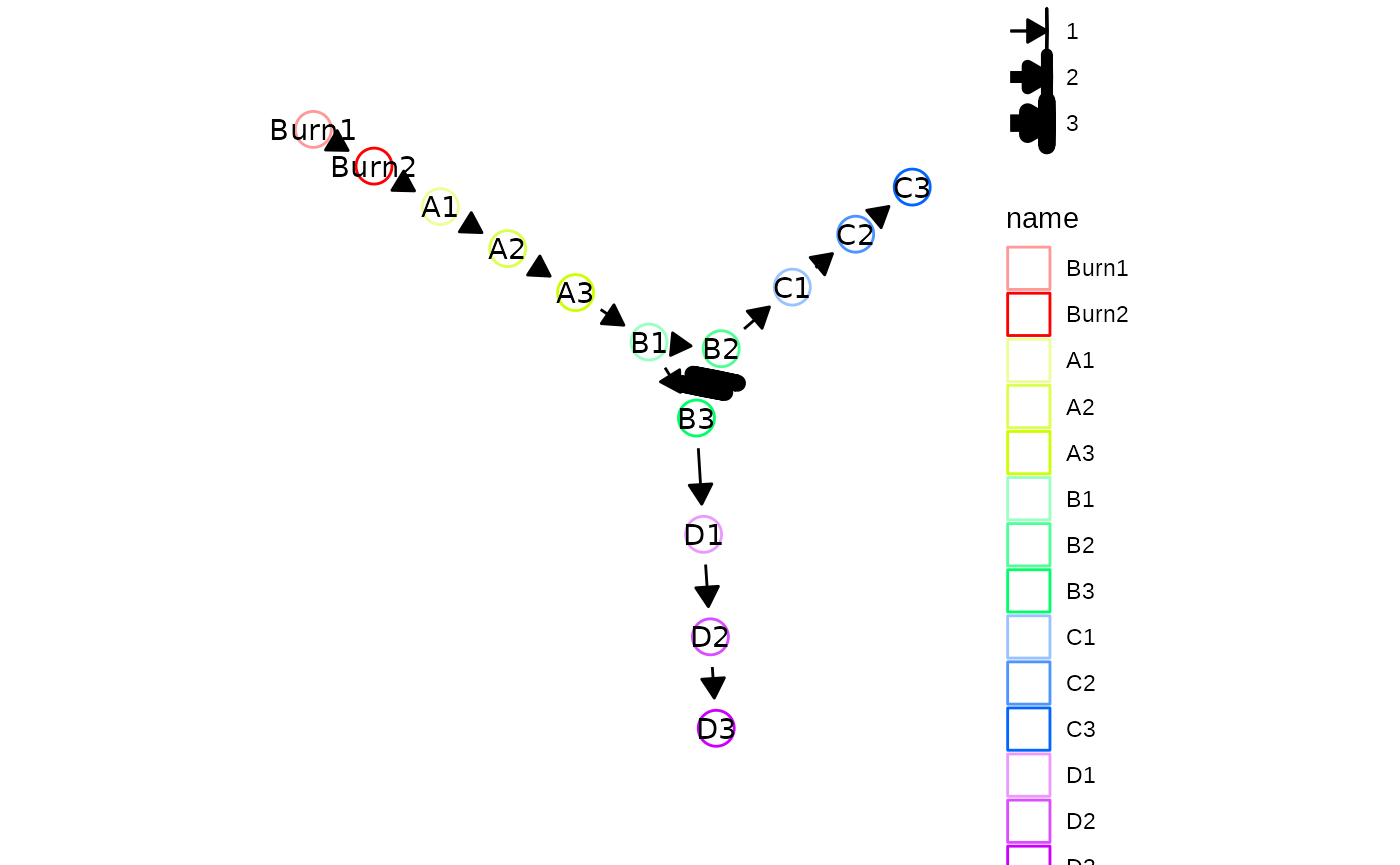

plot_backbone_statenet(config)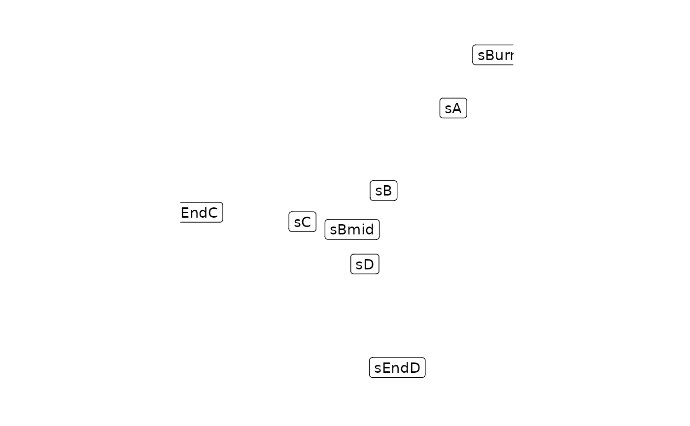

# the simulation is being sped up because rendering all vignettes with one core
# for pkgdown can otherwise take a very long time
config <- 
  initialise_model(
    backbone = backbone,
    num_tfs = nrow(backbone$module_info),
    num_targets = 50,
    num_hks = 50,
    verbose = interactive(),
    simulation_params = simulation_default(
      ssa_algorithm = ssa_etl(tau = .01),
      census_interval = 1,
      experiment_params = simulation_type_wild_type(num_simulations = 10),
      total_time = simtime_from_backbone(backbone) * 2
    ),
    download_cache_dir = tools::R_user_dir("dyngen", "data")
  )

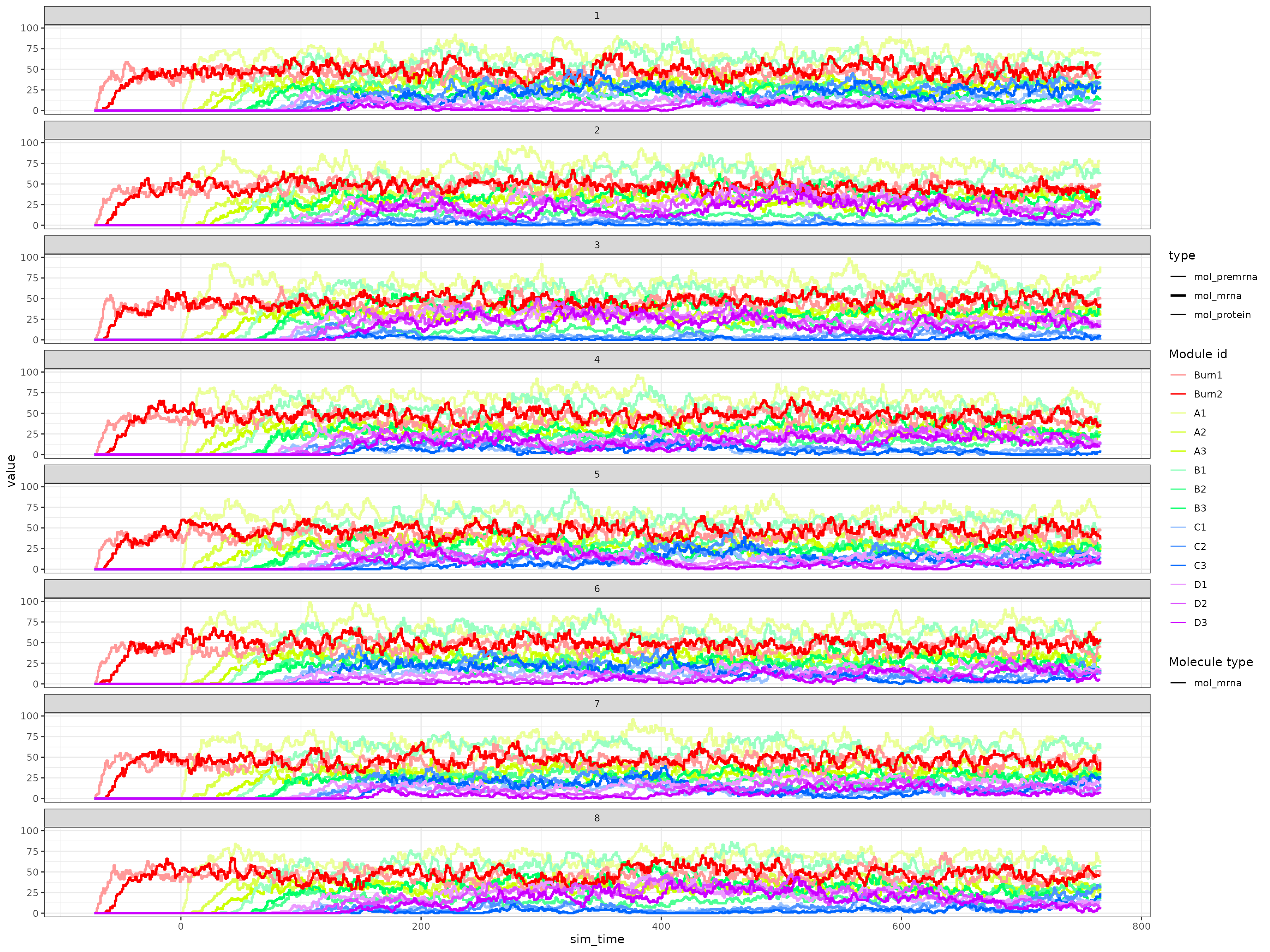
Looking at the gene expression over time shows that a simulation can indeed switch between C3 and D3 expression.

out <- generate_dataset(config, make_plots = TRUE)

print(out$plot)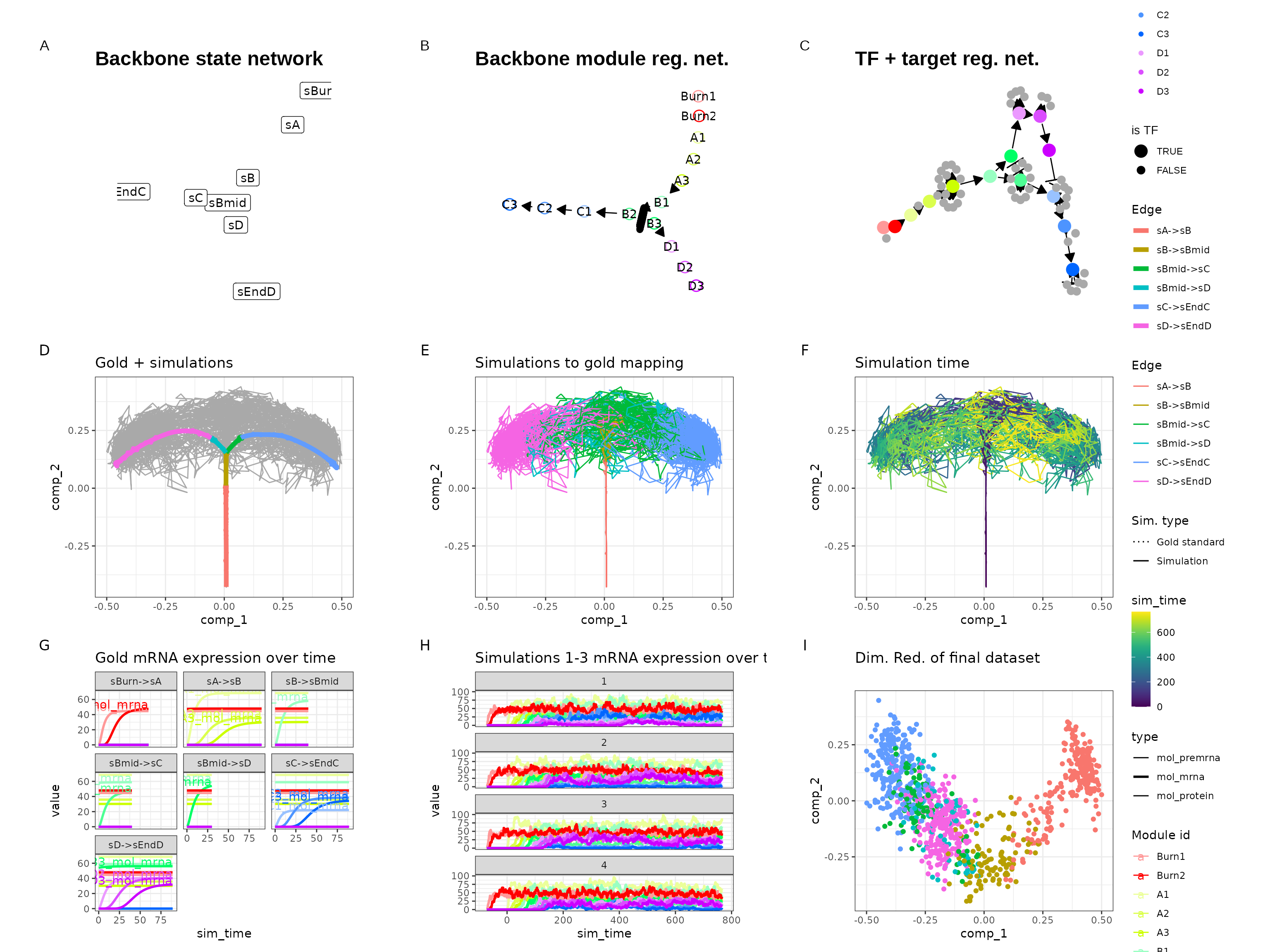

plot_simulation_expression(out$model, simulation_i = 1:8, what = "mol_mrna")