Advanced: Tweaking parameters

In some of the other vignettes, we tweak the values for census_interval and tau to speed up dyngen simulations. In this vignette, we demonstrate what happens when some of the commonly tweaked parameters are pushed too far.

Initial run

Let’s start off with a simple bifurcating cycle run and default parameters.

library(dyngen)
library(tidyverse)

## ── Attaching packages ─────────────────────────────────────── tidyverse 1.3.2 ──
## ✔ ggplot2 3.3.6      ✔ purrr   0.3.5 
## ✔ tibble  3.1.8      ✔ dplyr   1.0.10
## ✔ tidyr   1.2.1      ✔ stringr 1.4.1 
## ✔ readr   2.1.3      ✔ forcats 0.5.2 
## ── Conflicts ────────────────────────────────────────── tidyverse_conflicts() ──
## ✖ dplyr::filter() masks stats::filter()
## ✖ dplyr::lag()    masks stats::lag()

set.seed(1)

backbone <- backbone_cycle()

num_cells <- 500
num_features <- 100

# genes are divided up such that there are nrow(module_info) TFs and
# the rest is split between targets and HKs evenly.
num_tfs <- nrow(backbone$module_info)
num_targets <- round((num_features - num_tfs) / 2)
num_hks <- num_features - num_targets - num_tfs

run1_config <- 
  initialise_model(
    backbone = backbone,
    num_tfs = num_tfs,
    num_targets = num_targets,
    num_hks = num_hks,
    num_cells = num_cells,
    verbose = FALSE
  )

# the simulation is being sped up because rendering all vignettes with one core
# for pkgdown can otherwise take a very long time
set.seed(1)

run1_config <-
  initialise_model(
    backbone = backbone,
    num_tfs = num_tfs,
    num_targets = num_targets,
    num_hks = num_hks,
    num_cells = num_cells,
    verbose = interactive(),
    download_cache_dir = tools::R_user_dir("dyngen", "data"),
    simulation_params = simulation_default(
      census_interval = 5, 
      ssa_algorithm = ssa_etl(tau = 300/3600),
      experiment_params = simulation_type_wild_type(num_simulations = 10)
    )
  )

run1 <- generate_dataset(run1_config, make_plots = TRUE)

run1$plot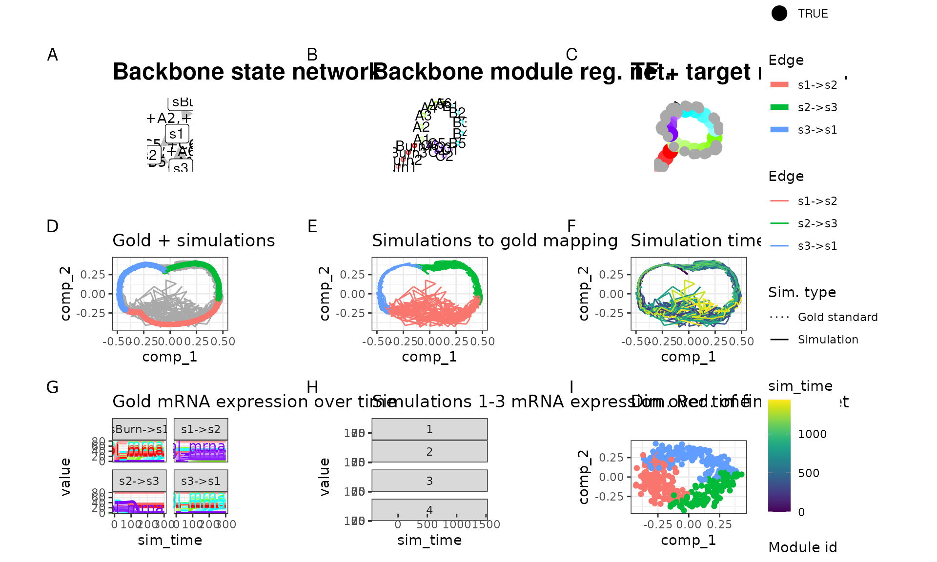

We tweaked some of the parameters by running this particular backbone once with num_cells = 100 and num_features = 100 and verifying that the new parameters still yield the desired outcome. The parameters we tweaked are:

On average, 10 cells are sampled per simulation (e.g. num_simulations = 100 and num_cells = 1000). You could increase this ratio to get a better cell count yield from a given set of simulations, but cells from the same simulation that are temporally close will have highly correlated expression profiles.
Increased time steps tau. This will make the Gillespie algorithm slighty faster but might result in unexpected artifacts in the simulated data.
census_interval increased from 4 to 10. This will cause dyngen to store an expression profile only every 10 time units. Since the total simulation time is xxx, each simulation will result in yyy data points. Note that on average only 10 data points are sampled per simulation.

Increasing time step `tau`

The tau parameter changes the size of the time steps made by dyngen during the simulation. Setting tau too large might cause certain production and degradation of molecules to fluctuate strangely.

run2_config <- 
  initialise_model(
    backbone = backbone,
    num_tfs = num_tfs,
    num_targets = num_targets,
    num_hks = num_hks,
    num_cells = num_cells,
    gold_standard_params = gold_standard_default(tau = 1),
    simulation_params = simulation_default(ssa_algorithm = ssa_etl(tau = 5)),
    verbose = FALSE
  )

# the simulation is being sped up because rendering all vignettes with one core
# for pkgdown can otherwise take a very long time
set.seed(1)

run2_config <-
  initialise_model(
    backbone = backbone,
    num_tfs = num_tfs,
    num_targets = num_targets,
    num_hks = num_hks,
    num_cells = num_cells,
    verbose = interactive(),
    download_cache_dir = tools::R_user_dir("dyngen", "data"),
    gold_standard_params = gold_standard_default(tau = 1),
    simulation_params = simulation_default(
      census_interval = 5, 
      ssa_algorithm = ssa_etl(tau = 5),
      experiment_params = simulation_type_wild_type(num_simulations = 10)
    )
  )

run2 <- generate_dataset(run2_config, make_plots = TRUE)

run2$plot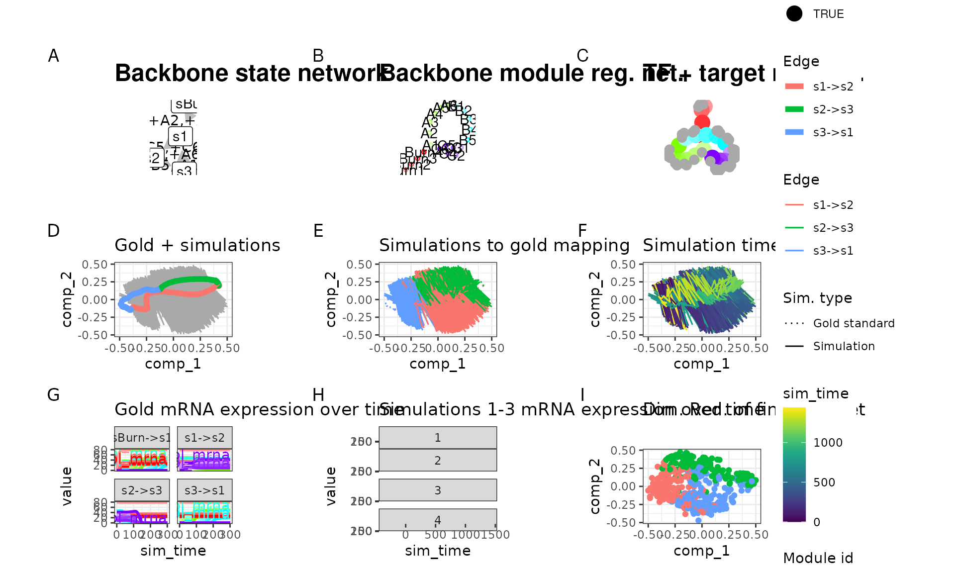

Certainly something strange is happening here. If we compare the expression values of the two runs, we can see that the second run produces much higher expression counts, but also at every step the high expression is lowered again.

plot_simulation_expression(run1$model, what = "mol_mrna", simulation_i = 1, facet = "none") + facet_wrap(~module_id)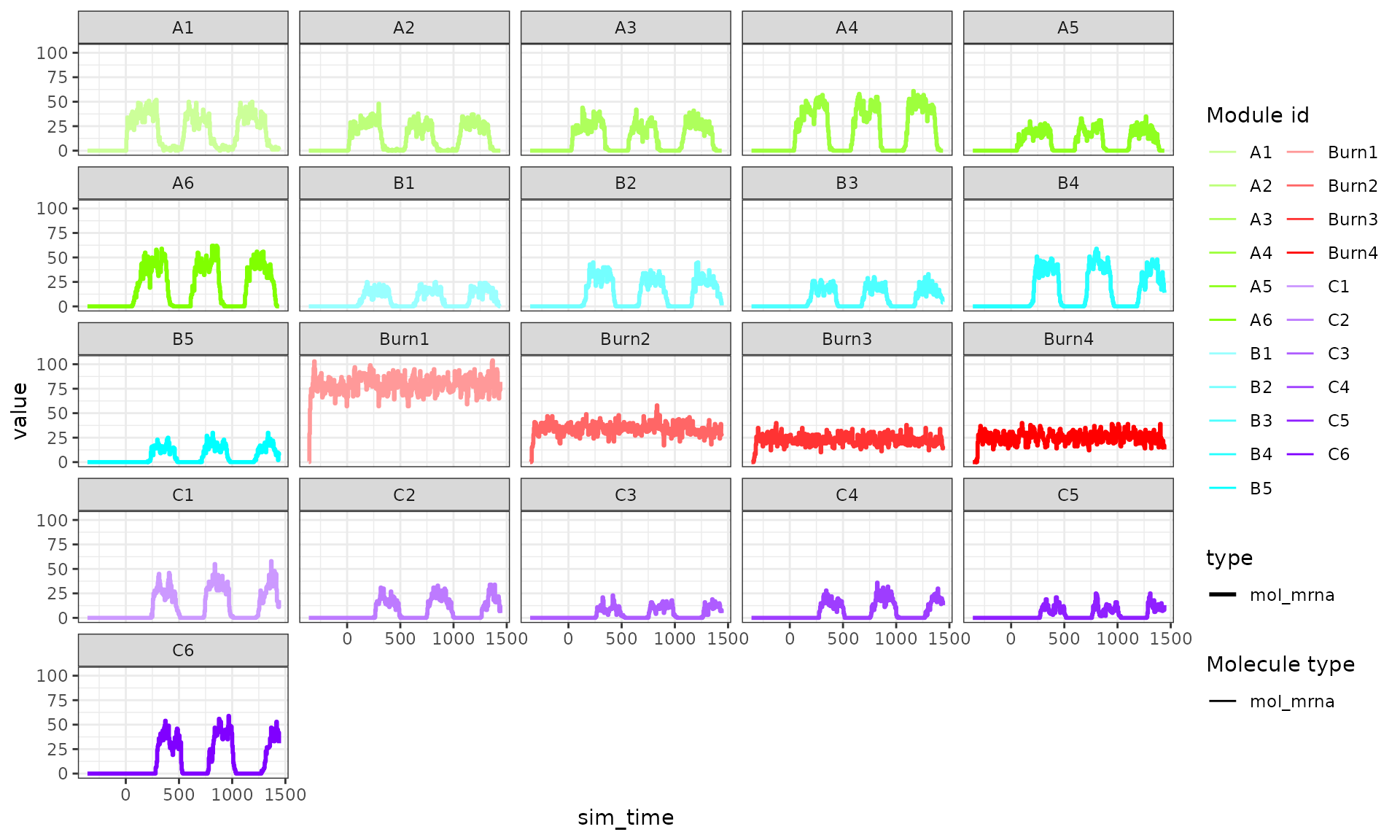

plot_simulation_expression(run2$model, what = "mol_mrna", simulation_i = 1, facet = "none") + facet_wrap(~module_id)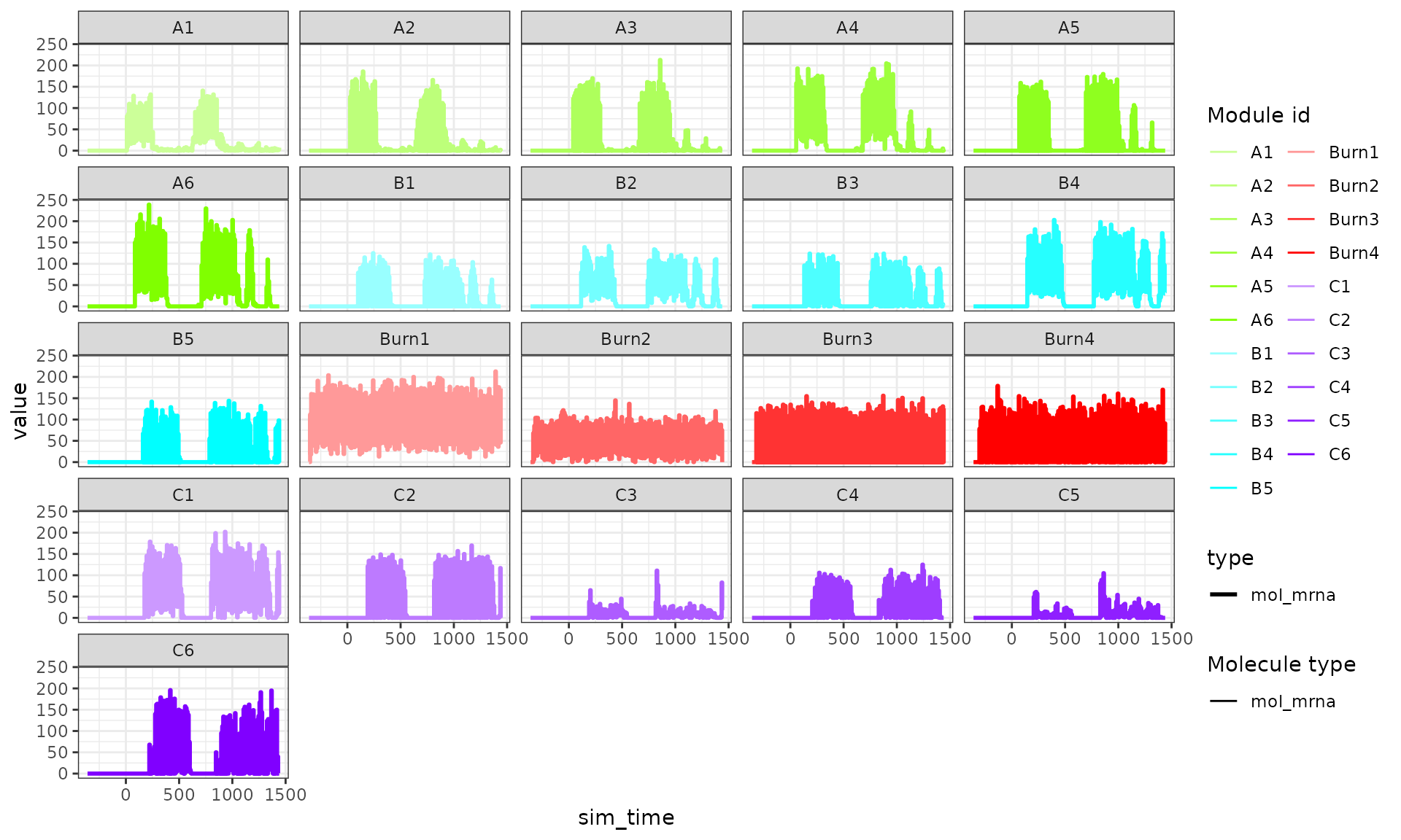

This is caused by setting tau too high; when the expression a gene is very low but the binding of a TF causes transcription to occur, transcripts will be created. However, at the start of a time step the gene is not expressed, so throughout the whole time step no degradation happen. In the next time step, however, there is a large number of transcripts, so these will quickly be degraded.

It’s recommended to set tau relatively low (e.g. 0.01). Setting it too low will cause the simulation to take a long time, however.

Controlling number of census generated

During a simulation of length total_time, dyngen will draw a census every with time steps of census_interval. The total number of census generated will thus be num_simulations * floor(total_time / census_interval). Ideally, the ratio between the number of census and the number of cells sampled from the census will be around 10. If this ratio is too high, dyngen will spend a lot of time comparing the census to the gold standard. If the ratio is too low, not enough census will be available for dyngen to draw cells from and a warning will be produced.

Controlling the ratio num_simulations * floor(total_time / census_interval) / num_cells can be performed by tweaking the census_interval.

run3_config <- 
  initialise_model(
    backbone = backbone,
    num_tfs = num_tfs,
    num_targets = num_targets,
    num_hks = num_hks,
    num_cells = 1000,
    gold_standard_params = gold_standard_default(
      census_interval = 100
    ),
    simulation_params = simulation_default(
      total_time = 1000,
      census_interval = 100,
      experiment_params = simulation_type_wild_type(
        num_simulations = 10
      )
    ),
    verbose = FALSE
  )

## Warning in initialise_model(backbone = backbone, num_tfs = num_tfs, num_targets = num_targets, : Simulations will not generate enough cells to draw num_cells from.
## Ideally, `floor(total_time / census_interval) * num_simulations / num_cells` should be larger than 10
## Lower the census interval or increase the number of simulations (with simulation_params$experiment_params).

In the example above, dyngen will sample each of the 10 simulations 10 times, resulting in only 100 census generated by dyngen. We can’t draw 1000 cells from 100 census, so dyngen will complain before even running the simulation.

Reference datasets: garbage in, garbage out

Reference expression datasets are used to modify the gene expression counts. If you want to mimic the expression characteristics of a specific single-cell platform you can provide your own reference datasets. Be aware that the Garbage In, Garbage Out applies – low quality reference datasets will negatively impact the final dataset created.

reference_dataset <- Matrix::rsparsematrix(
  nrow = 1000, 
  ncol = 1000, 
  density = .01, 
  rand.x = function(n) rbinom(n, 20, .1)
) %>% Matrix::drop0()

run4_config <- 
  initialise_model(
    backbone = backbone,
    num_tfs = num_tfs,
    num_targets = num_targets,
    num_hks = num_hks,
    num_cells = num_cells,
    experiment_params = experiment_snapshot(
      realcount = reference_dataset
    ),
    verbose = FALSE
  )

# the simulation is being sped up because rendering all vignettes with one core
# for pkgdown can otherwise take a very long time
set.seed(1)

run4_config <-
  initialise_model(
    backbone = backbone,
    num_tfs = num_tfs,
    num_targets = num_targets,
    num_hks = num_hks,
    num_cells = num_cells,
    verbose = interactive(),
    download_cache_dir = tools::R_user_dir("dyngen", "data"),
    simulation_params = simulation_default(
      census_interval = 5, 
      ssa_algorithm = ssa_etl(tau = 300/3600),
      experiment_params = simulation_type_wild_type(num_simulations = 10)
    ),
    experiment_params = experiment_snapshot(
      realcount = reference_dataset
    )
  )

run4 <- generate_dataset(run4_config, make_plots = TRUE)

run4$plot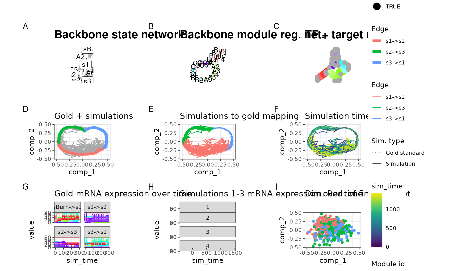

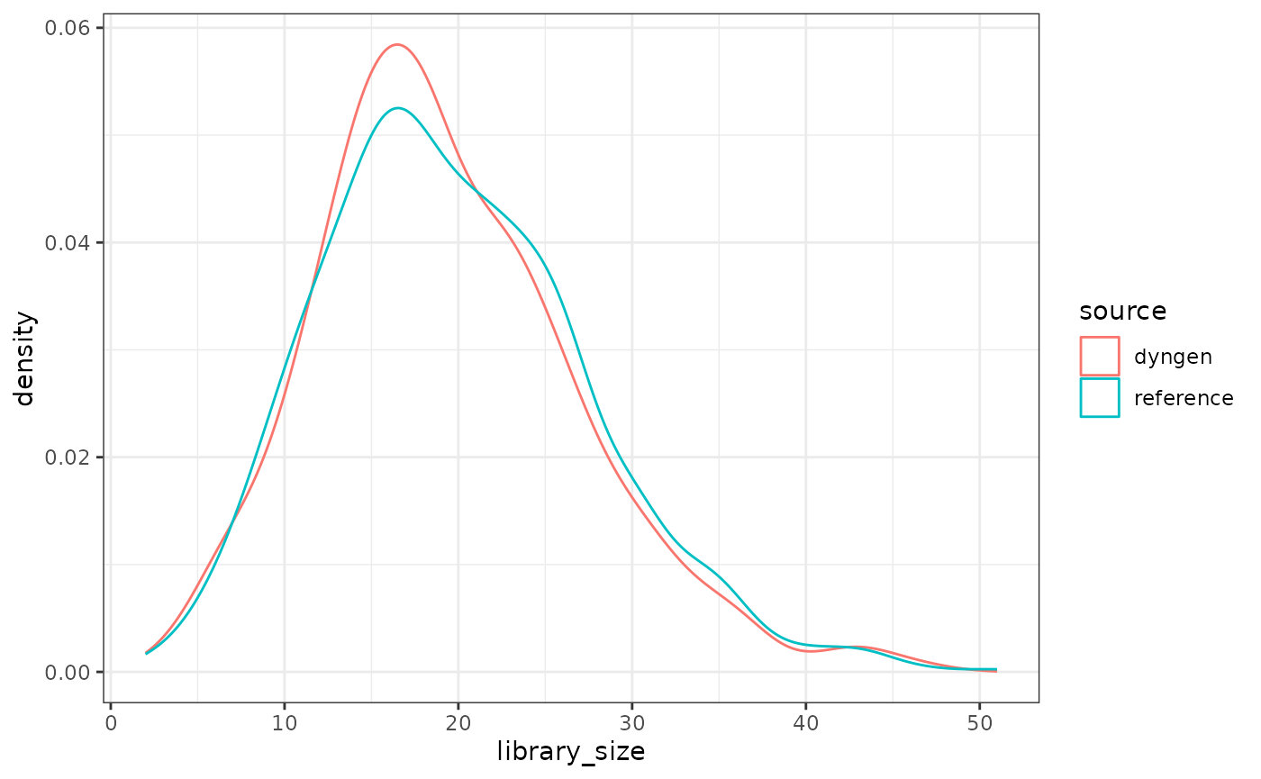
Notice how the last plot in the previous figure looks like total noise? This is because the reference dataset had very low library sizes for each of the ‘cells’ and dyngen attempts to match this as close as possible.

library_size_reference <- Matrix::rowSums(reference_dataset)
library_size_dyngen <- Matrix::rowSums(run4$dataset$counts)

dat <- bind_rows(
  tibble(source = "reference", library_size = library_size_reference),
  tibble(source = "dyngen", library_size = library_size_dyngen)
)
ggplot(dat) + geom_density(aes(library_size, colour = source)) + theme_bw()

Initial run

Increasing time step tau

Controlling number of census generated

Reference datasets: garbage in, garbage out

Increasing time step `tau`